An interesting walk from Bayesian statistics: Differences between MAP and MLE.

This article will allow you to understand the basis of any machine learning model. With simple words and few formulas, you will get fully proficency in Bayes, the Maximum Likelihood Estimation and the Maximum A Posteriori estimator.

Specifically, let’s start discussing about binary classification in terms of probability and discrimination functions. An interesting walk to understand the principles of machine learning algorithms beyond the facilities of scikit-learn and keras.

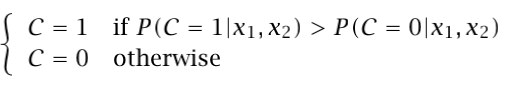
Imagine we have to classify cars in two families: eco and polluting. The information we have about the cars is the manufacturing year and the consumption, which we represent by two random variables X1 and X2. Of course, there are other factors which influence on the classification, but they are nonobservabable. Taking in mind what we can observe, the classification of a car is denoted by a Bernoulli random variable C (C=1 indicates eco, C=0 polluting) conditioned on the observables X=[X1,X2]. Thus, if we know P(C|X1,X2), when a new entry datapoint appears with X1=x1 and X2=x2, we would say:

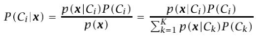
where the probability of error is 1-max(P(C=1|x1,x2),P(C=0|x1,x2)). Denoting x=[x1,x2] then we can use Bayes Theorem and it can be written as:

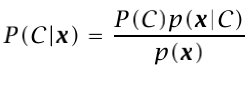
P(C) is called the prior probability because it is the information about C that we have in our dataset previous to analyze the observables x. As you have imagined, 1=P(C=1)+P(C=0).

P(x|C) is called the class likelihood because it is the probability that an event, which belongs to C=c, has the associated observation x.

P(x) is the evidence since it is the probability than an observation x is seen in our dataset. This term is also known as the normalization term since it divides the expression to get a value between 0 and 1. The evidence probability is the sum of all possible scenarios (also named as Law of total probability):

P(x)=P(x|C)1)P(C=1)+P(x|C=0)P(C=0)

Finally, P(C|x) is what we want to know, the probability of each class given an observation. This is called posterior probability as we classify it after seeing the observation x. Of course P(C=0|x)+P(C=1|x)=1.

In case of having several classes, we can extend this expression to K classes:

And the Bayes classifier will choose the class with the highest posterior probability P(Ci|x) from the K options.

In a previous article, I explained how to understand classification in terms of discrimination functions, which limit the hypothesis class region in the space. Following the same idea, we can implement that set of discriminant functions. Specifically, we choose C_i if:

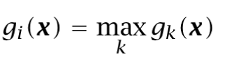
If we see the discriminant function as the Bayes classifier, the maximum discriminant function corresponds to the maximum posterior probability, obtaining:

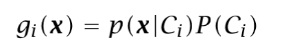
Please, observe that we have removed the normalization term (evidence) as it is the same for all discriminant functions. This set divides the feature space into K decision regions:

In practice, the pieces of information we observe, aka datapoints, they usually follow a given probability distribution which we represent as P(X=x) as we have discussed previously. Bayes classification seems easy to calculate when we have the values like P(C=1|x) or P(X=x). However, if we do not exactly know P(X), because we do not have access to all datapoints, we try to estimate it from the available information, and statistics come on stage.

A statistic is any value calculated from a given sample.

P(X) can have different shapes, but if the given sample is drawn from a known distribution, then we say it follows a parametric distribution. The parametric ones are quite desired because we can draw a complete distribution just knowing a couple of parameters. What do we do? Based on what we see (the sample), we estimate the parameters of the distribution by calculating statistics from the sample, the sufficient statistics of the distribution. This allows us to get an estimated distribution of our data, which we will use to make assumptions and take decisions.

Maximum Likelihood Estimation (MLE)

If you have reached this point, please forget everything about the previous Bayes explanation.

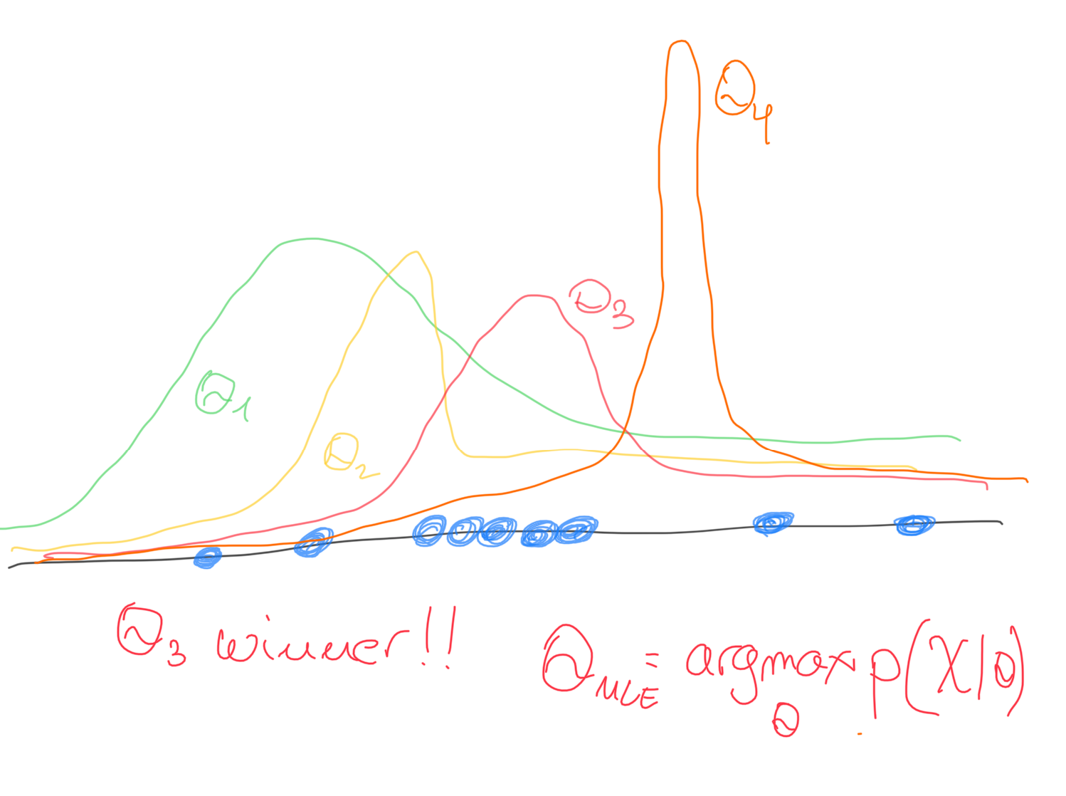
Let’s start from scratch: we have N datapoints in our dataset. It seems that the probability density of these datapoints follow a clear distribution family p(x), but we have no clue about the shape of the real distribution (its real center, its real dispersion, and so on). If we are facing a parametric distribution, it is as simple as calculating the parameters which define the real distribution. How? Let’s see the most likely option based on the given sample we have.

We have an independent and identically distributed (iid) sample:

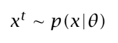
Its probability density is defined by a set of parameters θ. Let’s find the specific θ parameters that makes the distribution as likely as possible for the given sample. As the datapoints are independent amog them, their likelihood is the product of the likelihood of the individual points. Specifically, for a given θ, let’s see the probability p(x|θ). The higher probability, the higher match.

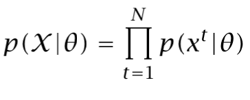
Then, the likelihood of θ for a given dataset X, l(θ|X) is equal to p(X|θ). In order to do things easier, we usually apply the log to the likelihood as the computations are faster (sums instead of multiplications):

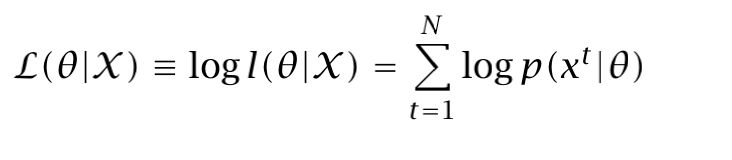
Now, we just have to drive the log likelihood, then maximizing it with regard to θ (for example using a Gradient Descent).

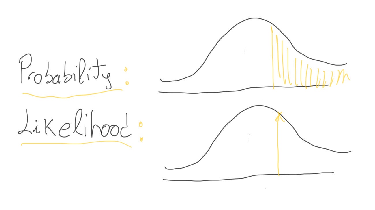
IMPORTANT NOTE: We usually interchange the terms "likelihood" and "probability". However, they are different things. The probability is the area under a fixed distribution (particular situation). With probability we want to know the chance of a situation given the distribution. In contrast, the likelihood is the y-axis value for a fixed point within a distribution that could be moved. Likelihood refers to finding the best distribution for a fixed value of some feature. The likelihood contains much less information about uncertainty, it is just a point instead of an area.

We run a search for different θ values, and we choose the θ that maximizes the log likelihood:

Image by author. Blue points represent the datapoints of the sample. Different distributions are drawn from different θ values, choosing the one with "the best match".

If we observe many different samples, the estimator of the parameters of the distribution will be more accurate and deviate less from the real parameters. Later we will see how to evaluate the quality of the estimators, in other words, how much the estimator is different from θ.

Applying MLE to a Bernoulli distribution

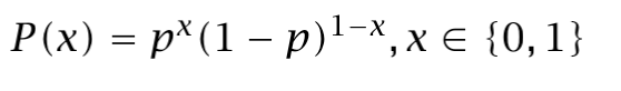
In Bernoulli, there are two possible states: true or false, yes or no. An event occurs or it doesn’t. Thus, each datapoint can take two values: 0 or 1. Actually, it takes the value 1 with probability p, and the value 0 with probability 1-p. Therefore:

The distribution is modeled with a single parameter: p. Thus, we want to calculate its estimator p̂ from a sample. Let’s calculate its log likelihood in terms of p:

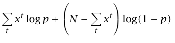
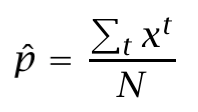
And now, solving dL/dp=0 in order to obtain the p̂ which maximizes the expression:

Maximum A Posteriori (MAP)

Now it is time to come back to Bayes theory. Sometimes, we could have some information about the possible value range that parameters θ may take, before looking at the sample. This information can be very useful when the sample is small.

Thus, the prior probability p(θ) defines the likely values that θ may take, previous to look at the sample. If we want to know the likely θ values after looking at the X sample, p(θ|X), we can use Bayes:

Note: We can ignore the normalizing term (or evidence), when we are talking about optimization, it does not affect.

Thus, if we want a model to predict an output for a given input x, y=g(x), as in regression, we really calculate y=g(x|θ). As it depends on the distribution.

However, since we do not know the real value of θ, we would have to take an average over predictions using all possible values of _θ (_weighted by their probability):

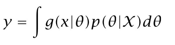
Evaluating an integral can be very complex and expensive. Instead of doing that, we can take just a single point, the most likely point, the maximum a posteriori.

Thus, we want to get the most likely value of θ, or in other words, maximize P(θ|X), which is the same as maximizing P(X|θ)P(θ):

If you take a second to compare this formula to the MLE equation, you can realize that it only differs in the inclusion of prior P(θ) in MAP. In other words, the likelihood is weighted with the information which comes from the prior. The MLE is a special case of MAP with no prior information.

The MLE is a special case of MAP.

If this prior information is constant (a uniform distribution), it is not contributing to the maximization, and we would have the MLE formula.

Specifically, imagine that θ can take six different values. Thus, P(θ) is 1/6 everywhere in the distribution:

However, if the prior is not constant (it depends on the region of the distribution), the probability is not constant neither and it has to be taken into account (for example, if the prior is Gaussian).

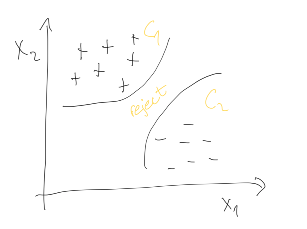
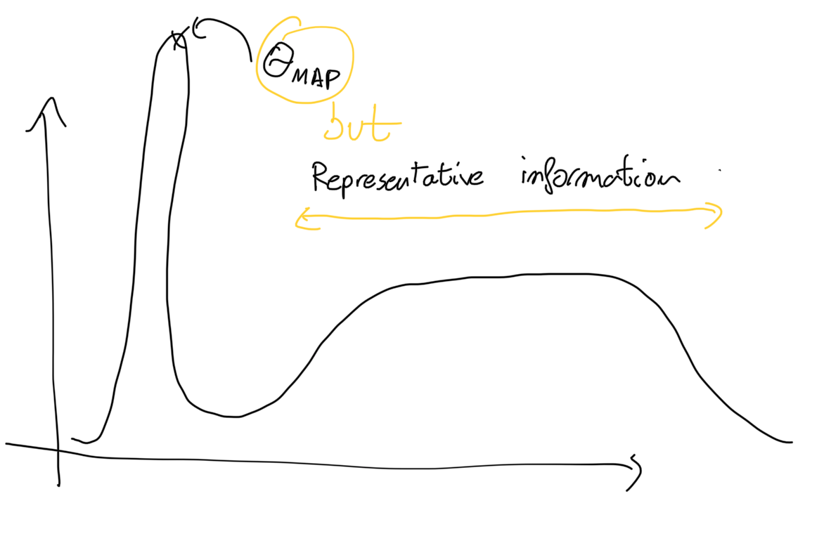
IMPORTANT: The maximum a posteriori can be chosen instead of computing the integral, only if we can assume that P(θ|X) has a narrow peak around its mode. Why? Because we are taking a single point, instead of computing all the region, and there is no representation of uncertainty. It may happen things like this when there is no a narrow peak around the mode:

Bibliography:

[1] Agustinus Kristiadi’s Blog https://wiseodd.github.io/techblog/2017/01/01/mle-vs-map/
[2] Ethem Alpaydin. Introduction to Machine Learning, 4th edition.