
Machine learning underlies the coolest technologies of today. This is how Ethem Alpaydin starts the Preface of his book, "Introduction to Machine Learning", which I had to read some years ago when I started with the Data Science world. Today, the book is still considered as a bible in the academic. The difference with many of the books you can find in Amazon is that it does not speak about technology, it only shows the algorithmic part of the Machine Learning. This is the point. Most people who work today with machine learning, they just use technology but have no idea about the mathematical basis of the algorithms that this technology encapsulates. It is very simple to call the ‘LDA’ algorithm in python on a pandas dataframe; but is even easier to execute a linear regression with caret on a R dataframe. This is fine if you need to build a model with some accuracy; but if you want to really explote your resources, you really need to completely understand the algorithms and maths behind the library or package you employ.
I write Medium stories because it is a straightforward way to review concepts and do not forget them. Thus, I am going to write a couple of series about the maths behind Machine Learning, starting with Supervised Learning. Do not worry, I know that theory is boring, so I will combine both theory with practical tips in order to do it as helpful as possible.
What is Supervised Learning? How is possible?
All of us know that an algorithm is a sequence of orders which allow to transform an input into one output. However, it happens many times that we have no idea about the orders or instructions needed to transform the input into the output; we are not able to build the algorithm despite of years of research. What we do is to learn to do the task, even if we do not the exact steps of the algorithm. Our approach starts with a very general model based on different parameters, and we will see how well the model approximates the output with those parameters. The learning passes through refining the parameters until finding the most accurate output. Learning corresponds to adjust the values of those parameters. We know that we cannot build the perfect approach, but yes a good and useful approximation.
In the process, there is a statistical perspective, since the core task is making inferences from a sample of available data: get parameters that better suit for those sample of data, creates a model based on those parameters and extrapolated that model for the global case.
The model can be predictive or descriptive, depending on if we want to make predictions or to gain explainability from data. With this, we are able to build different applications: Association Rules, Classification tasks, Regression, Pattern Recognition, Knowledge Extraction, Compression or Outlier detection, among many others.
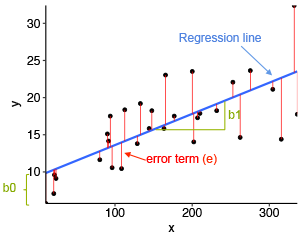
Both regression and classifications are supervised learning. The standard shorthand is to refer the input variables as X and the output variables as Y (a number in regression and a class code in classification). The task is to learn the mapping from X to Y, and we assume we can do it thanks to a model defined up to a set of parameters: Y=G(X|P) where G(·) is the model and P the parameters. During the learning process the machine learning algorithm optimizes the parameters in order to minimize the error, trying to be as close as possible to the correct values.
Before continuing, there is an important note here: the difference between Machine Learning algorithms and models, since it seems we can use both concepts interchangeably. The model is the final representation learned from the specific data with a specific and defined parameters; while the algorithm is the process to build that model: Model=Algorithm(Data). Linear regression is a machine learning algorithm; but y=3×1+3×2+1 is a model.
Parametric vs Nonparametric. Supervised vs Unsupervised
From the previous section, we use a learning target function G(·) that best maps input variables X to an output Y, trying to represent the real function F(·) which we do not know and we try to approximate. If we knew how F(·) looks like, we would use it directly and we would skip the learning phase.
Y=G(X)+E
There is an error E in our estimations, our model is accurate but not perfect. This error can have up to three different components: Bias error, variance error and irreductible error. We will see them later.
Parametric vs Nonparametric
In parametric algorithms, we map the model to a form, while nonparametric algorithms can learn any mapping from inputs to outputs.
In the case of parametric algorithms, we are assuming the form. This simplifies the process, but it is also limiting what it can learn. So we have to decide which form the model will have and then look for the parameters for such form. In the case of linear regression we are saying to the algorithm: "hey dude, you will learn something with this form: Y=B2X2 + B1X1+ B0", and the algorithm will look for the B2, B1 and B0 parameters that minimize the error of that expression on the given data. Other examples of parametric algorithms are LDA or Logistic Regression. The advantages are clear: simpler, faster and less data required. The withdraws are that you are forcing the model to fit a form that maybe it is not the best one for your case, and therefore the accuracy is poorer.
In contrast, the nonparametric algorithms are free to learn the shape, they do not require previous knowledge (SVM, Random Forest, Bayes, DNN), but of course they will require more data and there is higher risk of overfitting to the training data.
Supervised vs Unsupervised
The difference between these two kinds of algorithms is clear: if you have the real output with which you can compare the accuracy during the training, then it is supervised learning (you can answer how well did I do my estimation?); but if you have no clue about the output, then it is unsupervised learning (Does this person fit better to the cluster 1 or to the cluster 2? Anyone can tell me the real cluster of this person?).
In the case of supervised learning, we have a reference about how good is our model, as we have a target output with which compare during the training. The learning stops when it reaches an acceptable accuracy with respect to the given outputs of the training data. However, with the unsupervised algorithms, you only have the input data (X) but no an output target; so there is no way to calculate the accuracy of your estimations. This happens when clustering or finding association rules (HDBScan, Apriori, k-medoids).
Bias, Variance and Irreductible Errors in Supervised algorithms
Some paragraphs above, we saw that Y=G(X)+E in supervising learning. These supervised algorithms can be seen as a trade-off between bias and variance. Bias is the error assumptions we do when we say that the model has to fit a specific form. This makes the problem easier to solve. Variance is the sensitivity of a model to the training data.
In supervising learning, an algorithm learns a model from training data. We estimate G(·) from the training data, and G(·) is almost Y, but there is an error E. This error can be split into: bias error, variance error and irreductible error.
Irreductible error. It always happens despite of the data set you use for training or the algorithm you choose. This error is caused by external factors like hidden variables. You always have this error regardless all the effort you can do.
Bias error. The assumptions we do to make the G(·) function easier to learn. Thus, parametric algorithms have a higher bias. High bias makes algorithm faster to learn but less flexible. For example, Linear Regression and Logistic Regression are high-bias algorithms; while SVM or kNN are low-bias algorithms.
Variance error. How different our model is if we choose another portion of training data. Ideally, it shouldn’t change but it unfortunately changes in many cases. High-variance suggests that changes in the training dataset will largely change the G(·) function. Examples of high-variance algorithms are: kNN and SVM.
As we cannot control the irreductible error, we will focus on the bias and variance error. Ideally, the goal is to get low bias and low variance. But it is difficult to achieve both, so we have to balance them. Parametric or linear algorithms often achieve high bias but low variance; while non-parametric or non-linear algorithms usually get low bias but high variance.
Overfitting and Underfitting
Our learning process is made by learning a G(·) function from training data, trying to inference general patterns from specific examples, in contrast to deduction which learns specific concepts from general rules. The final goal of machine learning is to generalize well from specific data to any other data from the problem domain.
On the one hand, overfitting means to learn from training data too much, but not generalizing well to other data. This is the most common problem in practice, since it takes the noise from the training. Overfitting is more common with nonparametric and nonlinear models (low bias). On the other hand, underfitting means to train our model with insufficient data. That is the reason why we usually iterates until reaching a certain degree of error.
In practice, we usually plot the evolution of the error for a training set in addition to the error for a test set. If we iterate too much, we will reach a point where the training error continues decreasing and decreasing, but suddenly the error of the test starts to grow. This is because the model is picking the noise from the training data over the iterations. The sweet point can be just before the test error starts to rise; however, we use resampling and a validation dataset in practice in order to find that sweet point.

Classification
So far, we have described different concepts you should know for understanding any machine learning analysis. Let’s analyze now the maths behind classification, one of the most important fields within machine learning.
When learning from training data, we would like to have a specific pattern shared by all A-class examples (aka positive examples) and none of the B-class examples (aka negative examples). For instance, we train our data with million of car descriptions, which say whether each description belongs to a family car or not. Our model has learnt and, after that, it is able to say if a car, that we have not seen before, is a family car or not, just based on the given description.
Imagine the following example, we have a dataset X which describes different car models. Each datapoint x is composed of two features x1,x2 which represent the price (x1) and the engine power (x2) for each car x. Some of these cars are familiar (red points) or they don’t (green points):

What we have to do is to find the C rectangle which discriminates red from green points. Specifically, we have to find the p1 and p2 values for the price (x1) and e1 and e2 values for the engine power (x2) which limit the C rectangle. In other words, to be a familiar car is the same as being plotted between p1<x1<p2 AND e1<x2<e2 for suitable values of p1,p2,e1 and e2. This equation represents H, the hypothesis class from which we believe C is drawn, namely, the set of possible rectangles (the algorithm). However, the learning finds the particular hypothesis/rectangle h (which belongs to H) specified by a particular set of p1, p2, e1 and e2 values (the model). So, the parametric learning starts from a hypothesis class H, and finds values for p1, p2, e1 and e2 based on the available data, creating a hypothesis h which is equal or closest to the real C. Pointing out that we restrict our search to this hypothesis class (we are forcing to draw a rectangle, but maybe the real C is a circle), introducing a bias. Additionally, please observe that if there was a green point inside C, it would be a false positive; while if there was a red point outside C, it would be a false negative.
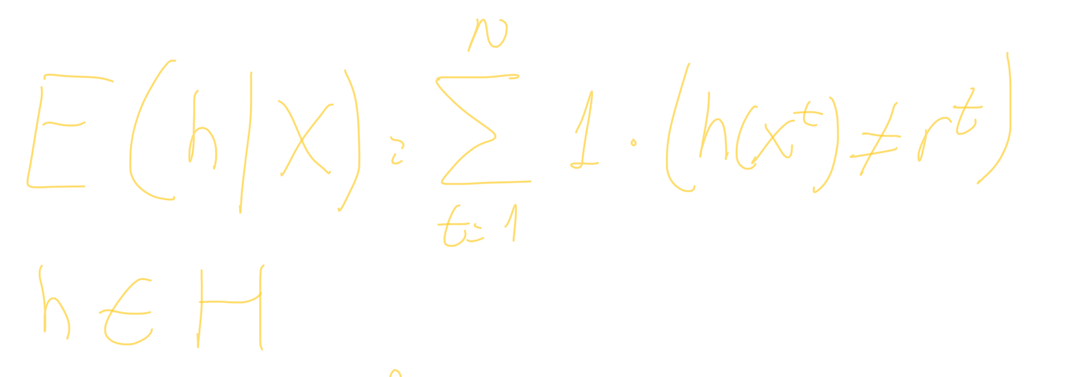
In real life, we do not know C. We have a dataset of data with the tag "it is familiar" or the tag "it is not familiar" for each vehicle x. This tag is named r. Then, we compare h(x) to r, and we see if they match or don’t. This is called the empirical error for a model h trained from a dataset X:
The question to be answered is how well will it classify future datapoints which are not included in the training set? This is the problem of generalization. Depending on how generous or restrictive we are for drawing our rectangle h when finding C, we could have the tightest rectangle S or the most general G:
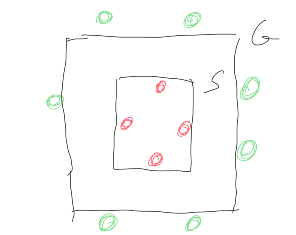
Any h from H between S and G are consistent with the training set. However, which would be better for future datapoints?
Depending on H and X, we will have different S and G. Let’s choose a h halfway between S and G. We define margin as the halfway distance from the boundary to the closest datapoint. So we choose the h with largest margin to balance the possibilites. The datapoints underlined in yellow define or support the margin:

We use an error (loss) function that, instead of checking whether an instance is on the correct class or not, it includes how far away it is from the boundary. In some critical applications, if there is any future instance which falls between S and G is a case of doubt, which is automatically discarded.
In the next article of this serie, we will review the Vapnik-Chervonenkis dimension, the Probably Approximately Correct learning, learning multiple classes and regression.
Adrian Perez works as Data Scientist and has a PhD in Parallel Algorithms for Supercomputing. You can checkout more about his Spanish and English content in his Medium profile.
Bibliography
Introduction to Machine Learning. Fourth Edition. Ethem Alpaydin. The MIT Press 2020.
Master Machine Learning Algorithms. PhD Jason Brownlee. 2016.


