How Does Socio-Educational Index Influence School Leaver Outcomes? – A Bayesian Analysis with R and brms

Following the very positive reception of the previous article seeking to understand if there is a proportional difference between school sectors and post-secondary outcomes, let’s follow up with a little more. We stated that the modelling was not intended to be causal, and is merely descriptive. This was prefaced by saying that there would be numerous factors that one might consider in a causal model. Well it so happens a proxy measure exists, ICSEA or Index of Community Socio-Educational Advantage.

A Bayesian Comparison of School Leaver Outcomes with R and brms

Continuing on from the previous article, we will seek to explore if there is a causal relationship between ICSEA across proportional outcomes by sector, amounting to a Bayesian ANCOVA workflow.

---

Background

Before jumping into the modelling, lets develop our causal model and understanding. ICSEA is a scale that identifies the socio-educational advantage of a school. This is a measure calculated by ACARA (Australian Curriculum Assessment Reporting Authority) that factors in parents educational background and occupation, Aboriginal status of students and the geographic location of the school. The average value of ICSEA is set to 1000 with a standard deviation of 100, and hence higher ICSEA values refer to schools with higher socio-educational advantage.

There are an enumerate number of factors that can affect student performance and outcomes. We’ve simplified to something more tangible below. Starting on the left hand side, we can reasonably expect a parents level of education to be an influence on their child’s personal ambitions, parental education will influence their salary, and hence what suburb they afford to live in, putting them proximal to schools within certain sectors. We are going to reasonably assume that affluent areas have a greater mix of Independent and Catholic schools ahead of Government schools. These are a lot of fields and data points to collate, summarise and create regression models to test our causal assumptions. Fortunately ICSEA is our magical proxy measure for most of these input variables, and thus on the right hand side we have our simplified causal model.

Academic literature has extensively explored this. One such review paper, available below by Alyahyan & Düştegör, provides a summary of an array of possible inputs that may influence academic success. We can see this is an incredibly complex set of relationships, across psychological, sociological, economic and environmental factors.

Predicting academic success in higher education: literature review and best practices …

Let’s not muddy the waters, because success is a subjective term derived from some preferred outcome.

Our research question is about understanding if there is a difference in outcomes across ICSEA levels between sectors, a subtle but important distinction.

Load Libraries and Datasets

ACARA is the Australian Curriculum Assessment Reporting Authority and they publish ICSEA and other performance indexes for all schools nationally here. This dataset is made available under CC BY 4.0. As before we’ll load data from the Victorian State Government’s On Track Survey of post-school leaver outcomes for students graduating in 2021, also available under CC BY 4.0

Below we do some rudimentary cleaning, and then join our two datasets profile and df_long to create df_longb, which contains our sector, outcome, proportions as previous as well as the corresponding ICSEA score for each school. Two schools didn’t have ICSEA scores so they have been removed.

library(tidyverse)
library(brms)
library(tidybayes)
library(readxl)
df <- read_excel("DestinationData2022.xlsx", 
    sheet = "SCHOOL PUBLICATION TABLE 2022", 
    skip = 3)
colnames(df) <- c('vcaa_code', 'school_name', 'sector', 'locality', 'total_completed_year12', 'on_track_consenters', 'respondants', 'bachelors', 'deferred', 'tafe', 'apprentice_trainee', 'employed', 'looking_for_work', 'other') 

df <- drop_na(df)

df2 <- df |> 
  mutate(across(5:14, ~ as.numeric(.x)), #convert all numeric fields captured as characters
         across(8:14, ~ .x/100 * respondants), #calculate counts from proportions
         across(8:14, ~ round(.x, 0)), #round to whole integers
         respondants = bachelors + deferred + tafe + apprentice_trainee + employed + looking_for_work + other, #recalculate total respondents
         filter(sector != 'A') #remove A schools (low volume)

df_long <- df2 |>
  select(sector, school_name, 7:14) |> 
  pivot_longer(c(-1, -2, -3), names_to = 'outcome', values_to = 'proportion') |> 
  mutate(proportion = proportion/respondants)

profile <- read_excel("school-profile-2022.xlsx", 
    sheet = "SchoolProfile 2022") |> #From ACARA
  filter(State == 'VIC' &amp; `School Type` %in% c('Secondary', 'Combined')) |> 
  select(`School Sector`, `School Name`, ICSEA, `ICSEA Percentile`) |> 
  drop_na() |> 
  mutate(`School Sector` = substr(`School Sector`, 1, 1),
         ICSEA_s = ((ICSEA - min(ICSEA-1)) / (max(ICSEA+1) - min(ICSEA-1))))

colnames(profile) <- c('sector', 'school_name', 'ICSEA', 'Percentile', 'ICSEA_s', 'percentile_d', 'percentile_c')

df_longb <-
  df_long |> 
  mutate(school_name = str_to_upper(school_name)) |> 
  left_join(profile |> mutate(school_name = str_to_upper(school_name))) |> 
  drop_na()

Exploratory Data Analysis

Our datasets are prepped and ready to go, lets visualise features of interest.

profile |> 
  ggplot(aes(y = sector, x = ICSEA, fill = sector)) +
    stat_halfeye(alpha = 0.5) +
    theme_ggdist() +
    scale_fill_viridis_d(begin = 0.4, end = 0.8) +
    labs(title = 'Distribution of ICSEA Values By Sector', y = 'Sector')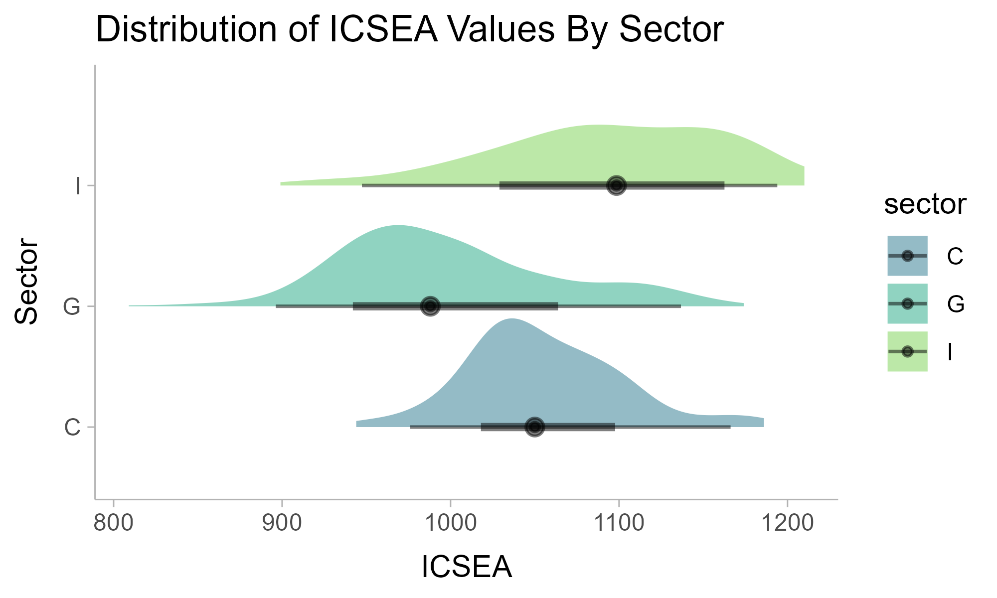

Interesting, and perhaps unsurprising is that public schools have the greatest variance, and independent schools with the highest median.

Bayesian ANOVA – Estimating Difference in Posterior Means of ICSEA

Let’s first examine if the difference between sectors amongst ICSEA is real, and like the previous article will conduct a Bayesian ANOVA. Also this begins to address the first part of our DAG, the relationship between ICSEA and Sector. We’ve instructed the model to provide parameter values for mu and phi for each level of sector.

m4e <- 
  brm(bf(ICSEA_s ~ sector + 0,
         phi ~ sector + 0),
      family = Beta,
      data = profile,
      prior = c(prior(normal(-1, 2), class = 'b'),
                prior(gamma(6, 2), class = b, dpar = phi, lb = 1)),
      seed = 246, warmup = 1000, iter = 6000, cores = 4, chains = 4, save_pars = save_pars(all = T)) |> 
  add_criterion(c('waic', 'loo'), moment_match = T)

summary(m4e)

We made a decision to rescale ICSEA using min-max so that we could model this using a Beta likelihood function, and thus the mu and phi parameters use logit and log link functions respectively.

Effectively the beta terms of the mean will be the logit value of the mean percentile for each sector, given rescaled ICSEA values.

Let’s briefly perform a posterior predictive check of each sector to see if the model is capturing as much of the observed data as reasonable.

alt_df <- profile |> 
  select(sector, ICSEA) |> 
  mutate(y = 'y', 
         draw = 99)

sim_df <- tibble(sector = c('C', 'I', 'G')) |> 
  add_predicted_draws(m4e, ndraws = 1200, seed = 246) |> #generates 1200 posterior draws for each sector
  mutate(ICSEA = (.prediction * (1211 - 808) + 808)) |> #rescale ICSEA back
  ungroup() |> 
  mutate(y = 'y_rep',
         draw = rep(seq(from = 1, to = 20, length.out = 20), times = 180)) |> #draws 
  select(sector, ICSEA, draw, y) |> 
  bind_rows(alt_df)

sim_df |> 
  ggplot(aes(ICSEA, group = draw)) +
    geom_density(aes(color = y)) +
    facet_grid(~ sector) +
    scale_color_manual(name = '', 
                       values = c('y' = "darkblue",
                                  'y_rep' = "grey")) +
    theme_ggdist() +
    labs(y = 'Density', x = 'y', title = 'Distribution of Observed and Replicated Proportions by Sector', subtitle = 'Model = m4e - Non-Pooled Phi')

Our model is reasonably capturing the shape about each sectors ICSEA distribution. Lastly let’s ask the model to tell us what the mean ICSEA difference between each sector using Bayesian ANOVA.

new_df <- tibble(sector = c('I', 'G', 'C'))

epred_draws(m4d, newdata = new_df) |> 
  mutate(ICSEA = .epred * (1211 - 808) + 808) |> 
  compare_levels(ICSEA, by = sector, comparison = rlang::exprs(C - G, I - G, C - I)) |> 
    mutate(sector = fct_inorder(sector),
         sector = fct_shift(sector, -1), 
         sector = fct_rev(sector)) |> 
  ggplot(aes(x = ICSEA, y = sector, fill = sector)) +
      stat_halfeye() +
      geom_vline(xintercept = 0, lty = 2) + 
      theme_ggdist() +
      theme(legend.position = 'bottom') +
      scale_fill_viridis_d(begin = 0.4, end = 0.8) + 
      labs(x = 'Difference in Mean Posterior ICSEAS', y = 'Sector Comparison', title = 'Sector Comparison of Posterior Distributions of Mean ICSEAS')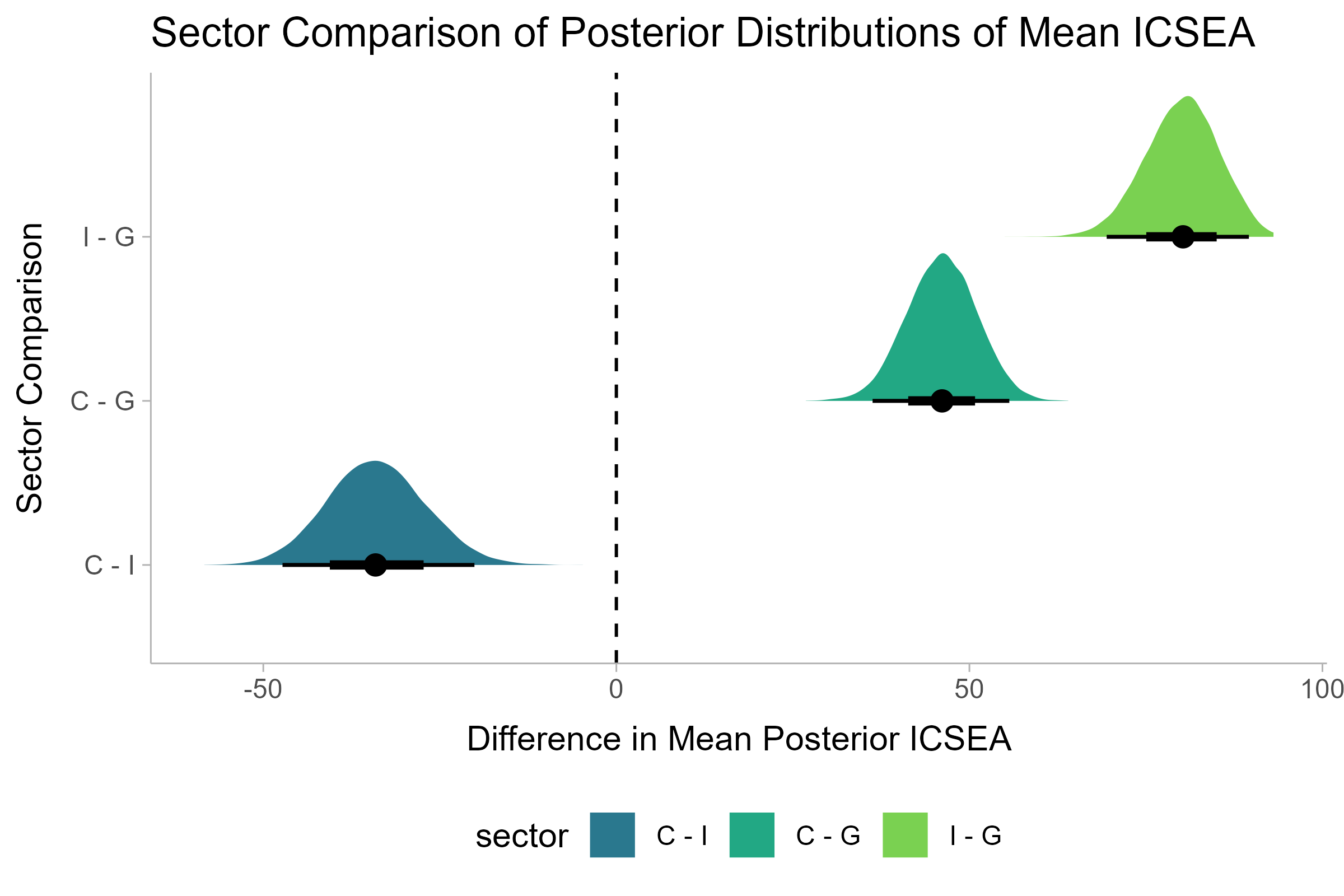

Given what we’ve observed above in our exploratory data analysis, these differences are not surprising. The average difference between Catholic and Government Schools is 46 points on the ICSEA scale, and 80 points between Independent and Government schools. The latter is almost a standard deviation away. Independent schools are on average 30 points higher then Catholic Schools. All these results are non-zero and real.

Bayesian ANCOVA – Impact of ICSEA on Proportional Outcomes by Sector.

Given we’d like to understand how much outcome proportions vary by ICSEA across and sector, we need to employ a hierarchical model. As our target variable is a proportion, we’ll continue using a Beta likelihood function.

We want to model the variation of ICSEA across sectors and proportional outcomes. This model took about 78 minutes to run on my machine using within-chain threading, so be warned. We’re not going to pretend to understand every single parameter in this model, we set broad general priors, and more importantly we are building a model that will enable us to answer the question.

m5d <- 
  brm(bf(proportion ~ 1 + (ICSEA_s|sector:outcome),
         phi ~ 1 + (ICSEA_s|sector:outcome)),
      family = Beta, 
      data = df_longb |> mutate(proportion = proportion + 0.01), 
      prior = c(prior(cauchy(0, 2), class = sd),
                prior(cauchy(0, 2), class = Intercept)),
      seed = 246, chains = 4, cores = 4, iter = 8000, warmup = 1000, save_pars = save_pars(all = T),
  control = list(adapt_delta = 0.99, max_treedepth = 15), threads = threading(2)) |> 
  add_criterion(c('waic', 'loo'), moment_match = T)

summary(m5d)

Let’s inspect the curve fit against the observed data.

new_df <- expand_grid(sector = c('C', 'I', 'G'),
            outcome = unique(df_long$outcome),
            ICSEA_s = seq(from = 0, to = 1, by = 0.05))

m5d |> 
epred_draws(new_df, ndraws = 200) |> 
  filter(outcome != 'other') |> 
  mutate(ICSEA = ICSEA_s * ((max(df_longb$ICSEA) + 1) - (min(df_longb$ICSEA) - 1)) + min(df_longb$ICSEA) - 1) |> 
  ggplot(aes(ICSEA, .epred, color = sector)) +
    stat_lineribbon() +
    geom_point(data = df_longb |> filter(outcome != 'other'), aes(y = proportion, x = ICSEA), alpha = 0.3) +
    facet_grid(sector ~ outcome) + 
    theme_ggdist() +
    theme(legend.position = 'bottom') +
    scale_color_viridis_d(begin = 0.2, end = 0.8) + 
    scale_fill_brewer(palette = "Greys") +
    labs(y = 'Proportion', x = 'ICSEA', title = 'Beta Regression Curve Fits of Proportion &amp; ICSEA by Sector and Outcome', subtitle = 'm5d Non-Pooled Phi Term')

The above tells an interesting story. Firstly, the proportion of students attending university post-high school demonstrates a positive trend with ICSEA, almost uniformly across sectors. Contrary to this, proportion of students in employment post high-school is negatively correlated with increasing ICSEA. The impact of ICSEA is now becoming a little more obvious, so lets understand the expected differences of proportional outcomes by ICSEA across sectors, ANCOVA.

new_df <- expand_grid(sector = c('C', 'I', 'G'),
            outcome = c('apprentice_trainee', 'bachelors', 'deferred', 'employed', 'looking_for_work', 'tafe'),
            ICSEA_s = seq(from = 0, to = 1, by = 0.05))

m5d |> 
epred_draws(new_df, ndraws = 2000, seed = 246) |> 
  compare_levels(variable = .epred, by = sector, comparison = rlang::exprs(C - G, I - G, C - I)) |> 
  mutate(ICSEA = ICSEA_s * ((max(df_longb$ICSEA) + 1) - (min(df_longb$ICSEA) - 1)) + min(df_longb$ICSEA) - 1,
         sector = fct_inorder(sector),
         sector = fct_shift(sector, -1), 
         sector = fct_rev(sector))  |> 
  ggplot(aes(y = .epred, x = ICSEA, color = sector)) +
    stat_lineribbon() +
    geom_hline(yintercept = c(0, -0.05, 0.05), lty = c(2)) +
    scale_fill_brewer(palette = "Greys") +
    scale_color_viridis_d(begin = 0.2, end = 0.8) + 
    facet_grid(outcome ~ sector, scales = 'free_y') +
    theme_ggdist() +
    theme(legend.position = 'bottom') +
    scale_y_continuous(labels = scales::label_percent()) +
    labs(x = 'ICSEA', y = 'Difference in Posterior Means', title = 'Sector Comparison of Outcomes by ICSEA')

The above tells an interesting story, and also highlights the benefit of a Bayesian approach – measuring uncertainty. Let’s hone in on the Bachelors outcome. At ICSEA levels below ~1000, Government schools on average have a higher proportion of students attending undergraduate education then both Independent and Catholic Schools.

Readers will be drawn to the narrowing of the difference in posterior means, between 1000–1100 ICSEA. Our estimates are more certain because there is general overlap in the schools in this space. Either side of these is reflected by a broadening of the uncertainty because of decreasing populations in the respective sectors, reinforced by our density plot above by sector and ICSEA.

Generally speaking the 50% of the posterior density largely resides between ±5% when conditioning on ICSEA for the bachelors outcome. This reinforces the positive relationship between ICSEA and school leavers attending some form of university education, with small bias towards Non-Government schools.

If we were to apply a ROPE (Region of Practical Equivalence) set to within ±5% of marginal differences, we could say that differences are indeed neglible.

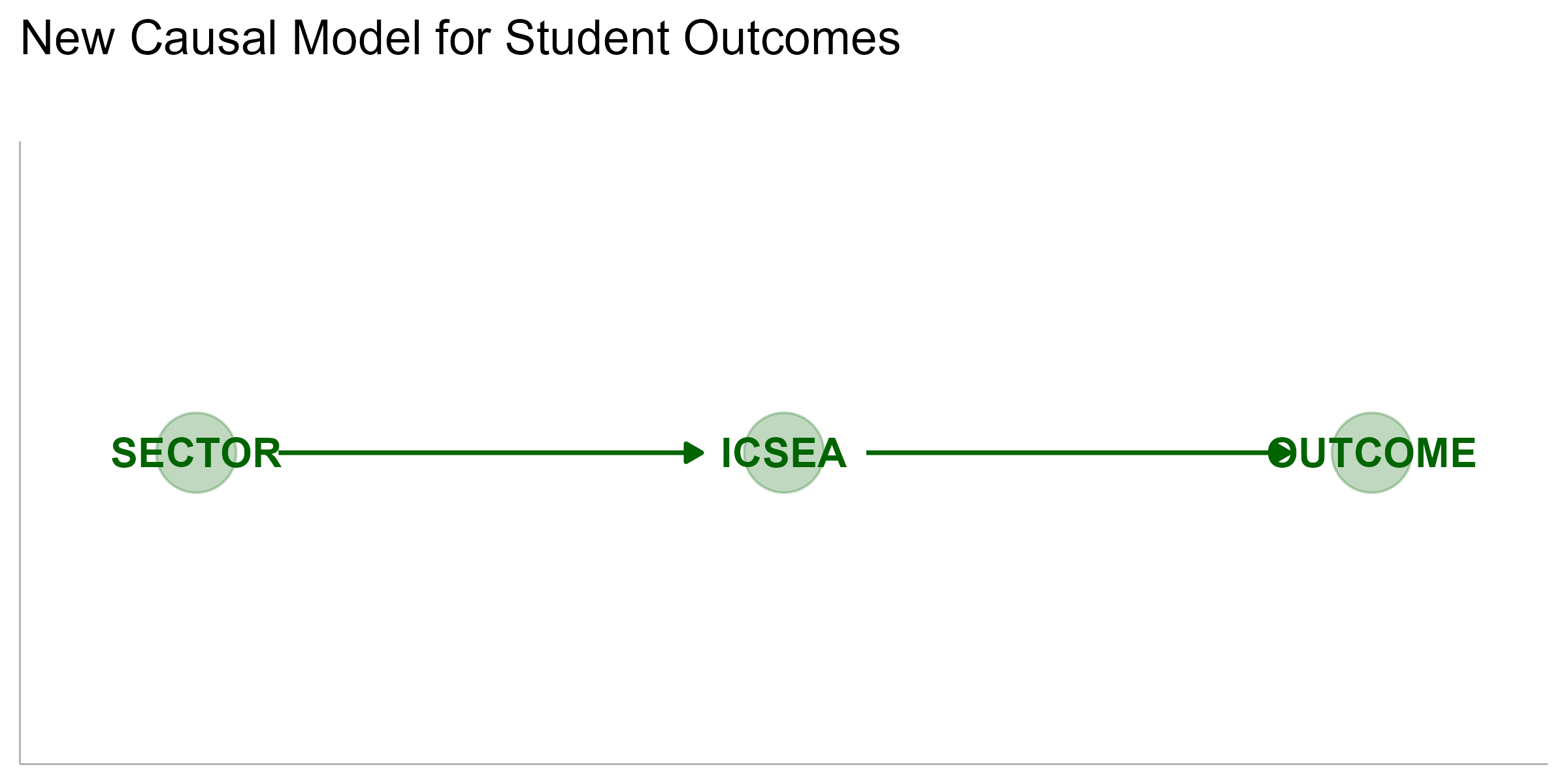
Evidenced by the differences in expected proportional outcomes by ICSEA, there is marginal difference across sectors when conditioning on ICSEA. Referring back to our causal DAG above, we can effectively reframe this from a Collider to a Pipe.

The outcome proportion is conditionally independent of sector when conditioning on ICSEA. Alternatively once we know the ICSEA of a school, the influence of sector is neglible within a ROPE of ±5% of mean posterior difference.

Outcome Proportion || Sector | ICSEA

Summary and Conclusion

In this article we have continued to explore secondary school leaver outcomes, this time incorporating the Index of Community Socio-Educational Advantage (ICSEA) as a scale that identifies the socio-educational advantage of a school as a proxy measure. We performed an initial Bayesian ANOVA to identify difference in posterior means of ICSEA across sectors. We then merged this with the outcomes dataset, performed a Bayesian ANCOVA to answer whether or not outcome proportion vary across sector when conditioning on ICSEA.

This work begins to reveal a possible causal model, which we’ve illustrated throughout with DAGs. Our conclusion, that Outcome Proportion || Sector | ICSEA is not unsurprising given what we understand about ICSEA. It was designed to capture an array of possible confounders in a single metric to describe a school or population level effect. For the purpose of this exercise it has allowed us to quantitate the mean differences across sectors, and found by in large to be neglible within ±5% ROPE.

References

1. Alyahyan, E., Düştegör, D. Predicting academic success in higher education: literature review and best practices. Int J Educ Technol High Educ 17, 3 (2020). https://doi.org/10.1186/s41239-020-0177-7