Shapley Values Clearly Explained

When was the last time you teamed up with some buddies and achieved something great together? Whether it was winning a game, mastering a project at work, or finishing in the top 3 in a Kaggle competition. And if you can’t remember anything (poor you), what about a nice evening with your friends? Picture this: a fantastic night out, followed by sharing a taxi ride home, only to be greeted with a sizable taxi bill. It’s in such moments that you may find yourself wondering:

How can we distribute our team result fairly across every member?

A team can also be the features of a Machine Learning model, the team’s outcome the prediction that the model makes. In this case, it is interesting to know how much each feature contributed to the final prediction. This is what data scientists are typically interested in.

Fair or even?

As an example, imagine that you teamed up for a competition with two more friends. You performed well and received 12,000 € as a team. How do you distribute the money fairly? Distributing it evenly is no problem, everybody gets 4,000€. But we all know that often some people contribute more to the team’s success than others. So maybe a split like 5,000€ + 4,000€ + 3,000€ would be more appropriate, depending on the circumstances.

Or take that taxi bill. You and two other friends went home after hanging out, and that taxi ride home cost you 60€ in total. Is it fair for everyone to pay 20€? Or isn’t it fairer if a person who lives really far away pays more than the ones who live closer, maybe even close together? And if this person has to pay more, how much more should it be?

---

In this article, I will show you how to answer questions like this using Shapley Values, named after the Nobel laureate Lloyd Shapley. They provide a mathematical framework for assigning a fair share of a team’s success to each contributing member.

Three gentlemen in a taxi

As a running example, let us use the taxi scenario I mentioned before. Here comes a slightly more fleshed-out story:

In the charming town of Luton, three British gentlemen from Oxford, Cambridge, and London, dressed in dapper suits, spent a jolly evening exploring its cobblestone streets. Starting at a local pub, they clinked glasses in celebration, moved on to the bustling marketplace for street food delights, and ended their night in a refined tearoom, sipping tea to the soothing tunes of a live pianist. With hearts warmed by laughter and shared moments, the trio bid farewell to Luton, leaving behind the echoes of a truly delightful evening.

What a lovely story, innit? In the end, the friends shared a single taxi – to spend some more time together – to get home.

As you can see, the taxi has to drive quite a route to go from Luton all the way around to reach all three cities. The taxi price was 3£/mile, and it went 161 miles, resulting in a price of 483£. Phew. But now comes the question of questions:

How much should everyone pay?

Let us start with a few observations.

1. London is closest to Luton, 34 miles.
2. If the London friend had gone home on his own, the other two friends would still have needed to travel 127 miles to get home, which is still quite a lot.

The same is not true for the other cities. Intuitively, this means that the friend going to London did not increase the mileage too much and should pay less compared to the other two. We will now learn how to compute the exact and fair numbers according to Shapley.

Computing Shapley Values

Everything we need to know to compute Shapley values is the prices for each combination – also known as coalition – of friends taking the taxi. Let us call the friends C(ambridge), L(ondon), and O(xford) from now. C, L, and O are also called players in general.

Coalition values

We have established that a coalition of C, L, and O would have cost 483£, this is what we have observed. We also write this as v({C, L, O}) = 483, meaning that the value of the coalition {C, L, O} is 483.

However, we did not observe any other coalition value. This is usually the case when you want to compute Shapley values. You have the value of the full coalition, but you have to come up with the other values as well. For example, what would have been the price if only C and O would have taken the taxi?

In our case, we can reconstruct these values using Google Maps. Visiting Cambridge and Oxford would have been a 127-mile ride that cost 127 miles · 3£/mile = 381£, so v({C, O}) = 381. As another example, take the coalition {L}, i.e., only going to London. That would have been a 34-mile ride from Luton, resulting in a coalition value (price) of v({L}) = 34 · 3 = 102.

You can do the same for all other coalitions and get the following list:

Contribution values

Now that we have this list, the idea of Shapley values revolves around the concept of contributions. As an example, let us find out how much C contributes. But what does contributing even mean?

Well, if the taxi is empty – with a cost of 0 – and C gets in, the price goes from 0 to 114 according to the table above. The contribution of C in this case is v({C}) – v({}) = 114 – 0 = 114.

As another example, if there is only O in the taxi — with a cost of 150 — and C joins him, the cost increases to 381. Hence the contribution in this case is v({C, O}) – v({O}) = 381 – 150 = 231.

The fair share that everyone has to pay should intuitively be connected to how much their presence in this coalition (taxi) contributes to the final value (price).

However, we have the following dilemma:

Contributions are heavily tied to the concept of time.

You can see this reflected in how we came up with the contributions for C.

• First, the taxi was empty, then C joined, driving up the price by 114 = v({C}) – v({}).
• First, only O was in the taxi, then C joined, driving up the price by 231 = v({C, O}) – v({O}).
• First, O and L were in the taxi, then C joined, driving up the price by 195 = v({C, L, O}) – v({L, O}).

But you only know that everyone was in that taxi, there is no inherent timely order. So, did C drive up the price by 114, 231, or 195? And here is the magic sauce to solve this dilemma:

Just average the contribution values over all potential orderings of the coalition in time.

Sounds abstract, but let us compute how it works for C.

Average over permutations

If we just know that C, L, and O were in the taxi, let us consider all orderings in which they could have entered it. Let us make another list!

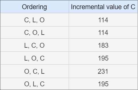
In the table above, you can see a lot of numbers that we have seen before. If C comes first, his incremental value is 114. The order of L and O afterward does not matter, it is 114 in both cases. Similarly, if C gets in last, his incremental value is 195. If C comes after O, it is 231. The only new number here is at L, C, O, i.e., the incremental value of C when only L was in the taxi before.

And now? Take the average! The result is the Shapley value of C:

So, the fair price according to the Shapley values would be 172£ for C. You can do the math for L and O as well and get

Note that the sum is equal to the total price: 483 = 172 + 119.5 + 191.5. This is not a coincidence, but a provable result called Efficiency. Shapley values would be useless without this property.

Python code

I have written some code to replicate the steps we have taken. This code is definitely not the fastest way to calculate Shapley values, but you should be able to follow along.

from itertools import permutations

# from the article, change it as you wish
coalition_values = {
    frozenset(): 0,
    frozenset("C"): 114,
    frozenset("L"): 102,
    frozenset("O"): 150,
    frozenset(("C", "L")): 285,
    frozenset(("C", "O")): 381,
    frozenset(("L", "O")): 288,
    frozenset(("C", "L", "O")): 483,
}

def compute_shapley_values(coalition_values, player):
    players = max(coalition_values, key=lambda x: len(x))
    contributions = []

    for permutation in permutations(players):
        player_index = permutation.index(player)
        coalition_before = frozenset(permutation[:player_index])  # excluding player
        coalition_after = frozenset(permutation[: player_index + 1])  # player joined coalition
        contributions.append(coalition_values[coalition_after] - coalition_values[coalition_before])

    return sum(contributions) / len(contributions)  # average, results in Shapley values

for player in ("C", "L", "O"):
    print(player, compute_shapley_values(coalition_values, player))

# Output:
# C 172.0
# L 119.5
# O 191.5

If n is the number of players, we loop over n! player permutations. Even for small values of n, such as 10, this is a huge number already: 3,628,800 iterations. This makes this implementation rather useless. Also, I store all values in lists before taking the average, so memory-wise, the above code only works for small instances as well.

The General Formula

Now that we know the single steps, let me give you the classical Shapley value formula:

Phew, that’s quite a mouthful, even with the knowledge we’ve gained over the course of the article. Let me annotate a few things here.

So, let us get started. N is the set of all players, in our example N = {C, L, O}, and n = |N| is the number of players. S is a coalition, such as {C, O}. You can see that we have coalition values of coalitions S with and without player i. Taking the difference gives us the contribution values. x! is the factorial function, i.e., x! = x · (x – 1) · (x – 2) · … · 2 · 1.

Multiplicity

Now, the only mystery is this multiplicity factor. To understand it, let us go back to our contribution table of C.

You can see how some numbers appear multiple times, namely 114 and 195. The numbers are the same since the order of all players before C and after C does not matter for the contribution values. For example, the orderings C, L, O and C, O, L have the same contribution value since both use the formula v({C}) – v({}). C comes first, the order after it does not matter. The same with L, O, C and O, L, C. C comes last, the order of everything before does not matter.

If there were two more players X and Y, the following orderings would also have the same contribution values:

• X, O, C, Y, L
• X, O, C, L, Y
• O, X, C, Y, L
• O, X, C, L, Y

C is in the third place, the order of what happens before and the order of what happens after does not matter. In any case, the contribution value is v({C, O, X}) – v({O, X}).

The multiplicity counts the number of permutations with the same contribution value.

The combinatorial argument goes as follows: There is an ordering of n players, and I want to compute the Shapley value of the player in position |S| + 1. Before this player, there are |S| other players, and there are |S|! ways to rearrange those. After this player, there are still n – |S| – 1 other players, which we can rearrange in (n – |S| – 1)! ways. We can freely combine both permutations, leading to |S|! · (n – |S| – 1)! orderings with the same contribution value, which is exactly the multiplicity factor in the Shapley formula.

As a numerical example, take the player example again with an ordering like X, O, C, Y, L. We care about the C. There are two ways to permute X and O, as well as two ways to permute Y and L, leading to a multiplicity of 2! · 2! = 4, which is why this list had a size of four.

Faster implementation

Here is a much better implementation. I used the variable names from the formula to make it easier to understand.

from itertools import combinations
from math import factorial

coalition_values = {
    frozenset(): 0,
    frozenset("C"): 114,
    frozenset("L"): 102,
    frozenset("O"): 150,
    frozenset(("C", "L")): 285,
    frozenset(("C", "O")): 381,
    frozenset(("L", "O")): 288,
    frozenset(("C", "L", "O")): 483,
}

def powerset(set_):
    """Create all subsets of a given set."""
    for k in range(len(set_) + 1):
        for subset in combinations(set_, k):
            yield set(subset)

def compute_shapley_values(coalition_values, i):
    N = max(coalition_values, key=lambda x: len(x))
    n = len(N)
    contribution = 0

    for S in powerset(N - {i}):
        multiplicity = factorial(len(S)) * factorial(n - len(S) - 1)
        coalition_before = frozenset(S)
        coalition_after = frozenset(S | {i})
        contribution += multiplicity * (coalition_values[coalition_after] - coalition_values[coalition_before])

    return contribution / factorial(n)

for player in ("C", "L", "O"):
    print(player, compute_shapley_values(coalition_values, player))

# Output:
# C 172.0
# L 119.5
# O 191.5

Since we enumerate over all subsets, this implementation loops over 2ⁿ / 2 sets. This is still bad, but not as horrible as the n! iterations as in the first implementation. For n = 10, there are only 512 iterations instead of over 3 million.

Properties of Shapley Values

Let us end this article with some important properties of Shapley value.

1. Efficiency: The sum of all players’ Shapley values equals the full coalition value. (Proof: Click here.)
2. Symmetry: If two players i and j have the same contribution values, i.e., v(S ∪ {i}) = v(S ∪ {j}) for all coalitions S not containing the players i and j, their Shapley values are also equal. (Proof: Both sums have the same summands, hence, the whole sum is equal.)
3. Linearity: If there are two games with coalition value functions v and w, then the Shapley value for a player i in the combined game v + w is equal to the sum of the Shapley values in the single games, i.e., ϕᵢ(v+w) = ϕᵢ(v) + ϕᵢ(w). (Proof: Take the Shapley formula from above and plug in v+w instead of v. Then you can separate the sum into two sums, which correspond to ϕᵢ(v) and ϕᵢ(w).)
4. Null Player: If a player i never contributes anything, their Shapley value is zero, i.e., if v(S ∪ {i}) = v(S) for each S not containing i, then ϕᵢ(v) = 0. (Proof: All contribution values v(S ∪ {i}) – v(S) are zero, so the whole sum is zero.)

Another interesting fact is that the Shapley values are the only values that satisfy the above four properties.

Conclusion

The problem of dividing a joint team effort fairly among the team members is a problem everyone knows from real life. We often fall back on simple solutions, such as dividing the pot of gold into equal parts. After all, it’s easy to do and it sounds fair on paper.

However, now you have a tool to compute actual fair shares for each member. At least if you can quantify all coalition values, which is the main obstacle to using Shapley values in practice, along with the exponential complexity of the calculation.

In a later post, we will look in more detail at the use of Shapley values in machine learning to break down model predictions.

---

I hope that you learned something new, interesting, and valuable today. Thanks for reading!

If you have any questions, write me on LinkedIn!

And if you want to dive deeper into the world of algorithms, give my new publication All About Algorithms a try! I’m still searching for writers!

All About Algorithms