TARNet and Dragonnet: Causal Inference Between S- And T-Learners

Building machine learning models is fairly easy nowadays, but often, making good predictions is not enough. On top, we want to make causal statements about interventions. Knowing with high accuracy that a customer will leave our company is good, but knowing what to do about it – for example sending a coupon – is much better. This is a bit more involved, and I explained the basics in my other article.

Easy Methods for Causal Inference

I recommend reading this article before you continue. I showed you how you can easily come to causal statements whenever your features form a sufficient adjustment set, which I will also assume for the rest of the article.

The estimation works using so-called meta-learners. Among them, there are the S- and the T-learners, each with their own set of disadvantages. In this article, I will show you another approach that can be seen as a tradeoff between these two meta-learners that can give you better results.

Recap: Meta-Learners

Let us assume that you have a dataset (X, t, y), where X denotes some features, t is a distinct binary treatment, and y is the outcome. Let us briefly recap how the S- and T-learners work and when they don’t perform well.

S-learner

If you use an S-learner, you fix a model M and train it on the dataset such that M(X, t) _ ≈_ y. Then, you compute

Treatment Effects = M(X, 1) – M(X, 0)

and that’s it.

The problem with this approach is that the mode could choose to ignore the feature t completely. This typically happens if you already have hundreds of features in X, and t drowns in this noise. If this happens, the treatment effects will all be zero, although there might be a causal relationship between the treatment t and the outcome y.

T-learner

Here, you fix two model _M_₀ and M₁, and train M₀ such that M₀(X₀) ≈ _y_₀ and M₁(X₁) ≈ y₁. Here, __ (X₀, y₀) and (X₁, y₁) are the subsets of the dataset (X, t, y) whe_r_e t = 0 a_n_d t = 1 respectively. Then, you compute

Treatment Effects = M₁(X) – M₀(X).

Here, a problem arises if one of the two datasets is too small. For example, if there are not many treatments, then (_X_₁, _y_₁) will be really small, and the model _M_₁ might not generalize well.

TARNet

TARNet – short for Treatment-Agnostic Representation Network – is a simple neural network architecture by Shalit et al. in their paper Estimating individual treatment effect: generalization bounds and algorithms. You can describe it shortly as an S-learner forced to use the treatment feature t because it is baked into the architecture. Here is how it works:

Note: In this article, I simplify their model a bit by dropping their metric IPM. Still, it works just fine. Image by the author. — **Note:** In this article, I simplify their model a bit by dropping their metric IPM. Still, it works just fine. Image by the author.

You can see that first, there are some feed-forward layers to preprocess the input. Then, t is explicitly used to decide which sub-network to choose on the right side. Note that we will only use this during training. If we have a trained model, we can use the model to output both versions at the same time – the prediction for t = 1 and t = 0 – and subtract them.

Implementation in TensorFlow

We will now learn how to implement it. If you know TensorFlow, you will see that it is straightforward and does not need much code. I will define a meta-model that does the following:

Take an input and process it with a common_model .
Take the result and process it via both the control_model and treatment_model .
Output the control_model result if t = 0, and the treatment_model output if t = 1.

import tensorflow as tf

class TARNet(tf.keras.Model):
    def __init__(self, common_model, control_model, treatment_model):
        super().__init__()
        self.common_model = common_model
        self.control_model = control_model
        self.treatment_model = treatment_model

    def call(self, inputs):
        x, t = inputs

        # Step 1
        split_point = common_model(x)

        # Step 2
        control = self.control_model(split_point)
        treatment = self.treatment_model(split_point)

        # Step 3
        concat = tf.concat([control, treatment], axis=1)
        indices = tf.concat([tf.reshape(tf.range(len(t)), (-1, 1)), t], axis=1)
        selected_output = tf.gather_nd(concat, indices)
        return selected_output

You can pass in any base models that you like. For example, if you have your features X and da dedicated treatment vector t , as well as the labels y , you can instantiate and fit it like this:

common_model = tf.keras.Sequential(
    [
        tf.keras.layers.Dense(10, activation="relu"),
        tf.keras.layers.Dense(10, activation="relu"),
    ],
)

treatment_model = tf.keras.Sequential(
    [
        tf.keras.layers.Dense(10, activation="relu"),
        tf.keras.layers.Dense(1),
    ],
)

control_model = tf.keras.Sequential(
    [
        tf.keras.layers.Dense(10, activation="relu"),
        tf.keras.layers.Dense(1),
    ],
)

tar = TARNet(common_model, treatment_model, control_model)
tar.compile(loss="mse")

tar.fit(x=(X, t), y=y, epochs=3)

Now, what’s better than a neural network with two heads? Right, a neural network with three heads!

Created by the author using Leonardo AI.

Dragonnet

Dragonnet is a neat little extension of TARNet developed by Shi et al. in the paper Adapting Neural Networks for the Estimation of Treatment Effects in 2019. It is based on the following intuition:

You don’t need X itself, but only the information of X that is relevant for predicting whether a treatment was given or not.

I know that this is very abstract, but since we did not cover the theory about causality to make this statement precise, I am not going to slap random formulas in your face. You can find them in the paper if you are interested.

The authors depict their method like this:

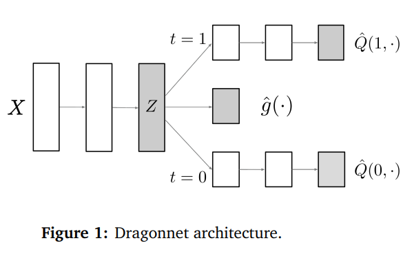
Here, g(x) = P(t = 1 | Z = z), i.e., the probability that a treatment was given, also known as propensity score. The Q‘s are the predictions for the cases t = 1 and t = 0 respectively, just like in TARNet.

If you want to see how to implement Dragonnet, you can find the authors’ version here.

This small change of adding a third head that computes the probability of getting treated regularizes the network in a way that it can estimate uplifts more robustly than before. The network is forced to distill a good representation Z of the original data X such that the middle head can make good predictions for the propensity score.

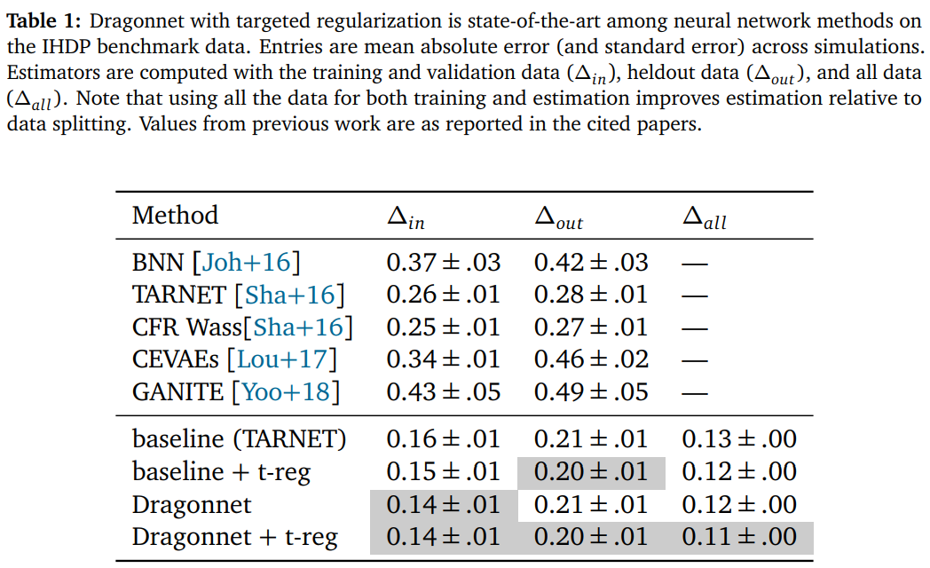
They quantify by doing experiments with synthetic data and summarize it as follows:

Conclusion

We have seen that the S- and T-learners can be viewed as two extremes for computing causal impacts. Both have their drawbacks and sometimes it can be beneficial to have something in the middle.

TARNet and Dragonnet fill in this gap – they function similarly to an S-Learner, but with a mechanism that forces them to use the treatment variable explicitly. This might lead to improved performance, but as so often: there is no free lunch, also in Causal Inference. There might be cases where the S- or T-learner performs best, but it is still important to know alternative approaches for uplift modeling.

I hope that you learned something new, interesting, and valuable today. Thanks for reading!