
Ah, time series forecasting. It’s the quintessential task for many data scientists, somewhat universal across various industries. This field is so valuable because if you have a crystal ball to see some key numbers ahead of time, you can use that information to get a head start and prepare for what’s coming down the pipeline.

Consider a call center: forecasting call volume allows for optimized staffing, ensuring efficient handling of customer inquiries. In retail, predicting when an item will go out of stock enables timely reordering, preventing lost sales and maximizing revenue. And of course, the holy grail of stock market prediction: if you could do this, you would be rich.
In this article, I want to show you how to do it the easy way using the awesome library sktime, the scikit-learn of time series forecasting.
Why Not Just Use scikit-learn?
Fair question! It’s kind of like asking, "Why use a fancy food processor when I have a knife and a cutting board?". Sure, you could chop everything by hand, but the food processor is designed specifically for that task and makes it way easier and faster. Let’s see how our food processor called sktime can help us.

Assume that we are given a history of data points y = (y(1), y(2), …, y(T)). We want to use them to predict the next time step y(T + 1). T might be today, and T + 1 the day tomorrow.
Modeling via regression
We can use standard Machine Learning techniques to create forecasts, but we have to rephrase the forecasting problem as a regression problem first. We have seen that in time series forecasting, we only use a vector y to predict another value, while in supervised machine learning, we need features and labels to train a model. Luckily, the translation is quite simple:

Here, we use a sliding window approach using the first three y values as features and the fourth as the label. These numbers of features and labels are hyperparameters that you can tune later.
Manual Implementation
It is straightforward to implement the logic from above:
import numpy as np

def reduce(time_series: np.ndarray, n_lags: int):
    X = []
    y = []

    for window_start in range(len(time_series) - n_lags):
        X.append(time_series[window_start : window_start + n_lags])
        y.append(time_series[window_start + n_lags])

    return np.array(X), np.array(y)
Here, I have just implemented the special case with a single label. You can use it like this:
ts = np.array([1, 2, 3, 4, 5, 6, 7, 8])
X, y = reduce(ts, n_lags=3)

print(X)
print(y)

# Output:
# [[1 2 3]
#  [2 3 4]
#  [3 4 5]
#  [4 5 6]
#  [5 6 7]]
#
# [4 5 6 7 8]
You can now take any supervised model you like and train it on (X, y). So, why do we need another library for that again? Well, in this easy case, everything is fine with our custom code, but if we want to:
- forecast several time steps with a special logic,
- preprocess the time series, or
- use time series methods that don’t rely on scikit-learn models
we’ll be thankful for Sktime’s flexibility. Let us see what I mean by that.
Introduction to sktime
I have told you now how awesome sktime is, but I still owe you the proof. So, let us express the sliding window logic and the model training with sktime’s syntax.
First example
Let us import some functionality and data. We will use the classical airline dataset created by Box & Jenkins that comes with sktime (BSD-3 license). It contains the monthly number of airline passengers over time, starting from January 1949. We want to extrapolate the passenger numbers into the future, so as an airline, we could deploy enough airplanes.
from sklearn.linear_model import LinearRegression
from sktime.datasets import load_airline
from sktime.forecasting.compose import make_reduction

y = load_airline()
Now, we can train the model using the sliding window approach like this:
ml_model = make_reduction(LinearRegression(), window_length=12)
ml_model.fit(y)
That’s it. We use a window length of 12 – meaning that we use the past 12 months to forecast the next one – because we can observe yearly seasonality. We can also tune this number, but 12 is good already. Now, sktime lets us create nice plots using the function plot_series :
from sktime.utils.plotting import plot_series

plot_series(
    y, # plot the history
    ml_model.predict(fh=np.arange(1, 13)), # plot the prediction
    labels=["History", "Forecast"]
)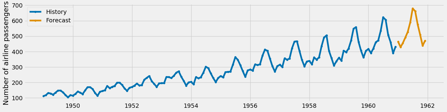
A few things to mention here. First, look how easy it is to make predictions. We can just call .predict and give it the (relative) time steps we are interested in. fh stand for forecasting horizon, and in order to forecast the next 12 months, we can set it to [1, 2, …, 11, 12].
The .predict method yields a pandas series with a consistent time index which enables the plot function to properly align the original time series and the forecast.
Under the hood
We have developed a linear regression model designed to predict just the subsequent time step. So, how have we forecasted twelve steps ahead? There are multiple methods to accomplish this, but sktime’s default method is recursive forecasting. Here is how it functions: Initially, we forecast the next time step, which is straightforward.

To predict the second one, we treat the first prediction we have created as an actual input.

Just repeat this process until you have created as many predictions as you need!
Note: I won’t go into great detail about the recursive approach. Just bear in mind that eventually, the model begins to make predictions based only on its previous forecasts, which might reduce the accuracy as we predict further ahead. sktime also offers other methods such as direct forecasting, which uses a separate model for each time step, and multiforecasting, where a single model predicts multiple time steps at once.
Classic time series models
If you want to try out classical models such as ARIMA, Exponential Smoothing (ETS), or TBATS, sktime got you covered as well. For example, if you want to train a triple exponential smoothing (Holt-Winters) with multiplicative trend and seasonality, you can do it like this:
from sktime.forecasting.exp_smoothing import ExponentialSmoothing

classical_model = ExponentialSmoothing(trend="mul", seasonal="mul")
classical_model.fit(y)
You can also plot the two forecasts in the same image, just to eyeball which one looks better.
plot_series(
    y,
    ml_model.predict(fh=np.arange(1, 37)),
    classical_model.predict(fh=np.arange(1, 37)),
    labels=["History", "ML Forecast", "ETS Forecast"]
)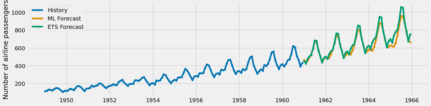
We observe that both forecasts begin somewhat similarly, but the peaks in the exponential smoothing (ETS) version appear to escalate more rapidly. In my view, both forecasts seem plausible; however, to determine which one is objectively better, we would need to conduct a more thorough analysis using performance metrics. Let’s do it!
Cross-validation
We can import some more functions and classes to measure performance properly.
from sktime.forecasting.model_evaluation import evaluate
from sktime.performance_metrics.forecasting import MeanSquaredError, MeanAbsolutePercentageError, MeanAbsoluteError
from sktime.split import ExpandingWindowSplitter

cv = ExpandingWindowSplitter(
    initial_window=36,
    step_length=12,
    fh=np.arange(1, 13)
)

metrics = [
    MeanAbsolutePercentageError(), # MAPE
    MeanSquaredError(square_root=True), # RMSE by setting square_root = True, otherwise MSE
    MeanAbsoluteError() # MAE
]

ml_evaluation = evaluate(ml_model, cv, y, scoring=metrics)
classical_evaluation = evaluate(classical_model, cv, y, scoring=metrics)
We evaluate it using an expanding window. It starts with a length of 36 months, we shift it by 12 months always, and we always predict 12 months ahead. Visually:
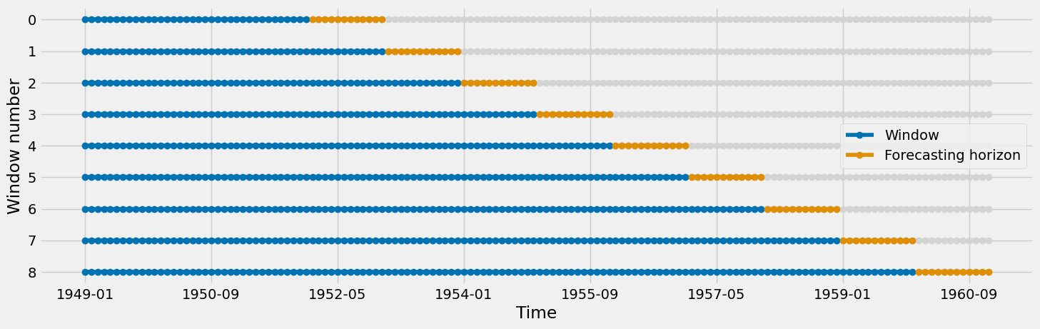
For these 9 different train-test splits, we get the following results for the linear regression model:

For each of the 9 splits, we can see MAPE, RMSE, and MAE on the test set. Furthermore, sktime gives the fit and prediction time durations as well as some information about the training dataset. Similarly, for the exponential smoothing model, we get:

Since it is a bit hard to parse, let us just take the mean per dataframe to boil down the information. If we visualize the RMSE and MAE, we get:

So, in this case, ETS wins. However, keep in mind that the linear regression model is not tuned. One fundamental hyperparameter to play around with is the window length. You can also use sktime for feature engineering, e.g., creating running means or standard deviations.
Conclusion
In this article, I have shown how simple it is to employ sktime for daily forecasting tasks. It is as user-friendly as scikit-learn, and you can even integrate your preferred scikit-learn models to make predictions!
However, we have only explored the basic features of sktime. In a future article, we will tackle:
- transforming target variables,
- utilizing pipelines,
- performing hyperparameter tuning,
- feature engineering,
- and much more.
Additionally, sktime provides tools for reconciling forecasts, which is useful when working with hierarchical time series. Find out more here:
I hope that you learned something new, interesting, and valuable today. Thanks for reading!
If you have any questions, write me on LinkedIn!
And if you want to dive deeper into the world of algorithms, give my new publication All About Algorithms a try! I’m still searching for writers!


