Advanced Time Series Forecasting With sktime

In my previous article, we explored the basics of time series forecasting with sktime, looking at how to leverage this powerful library for straightforward forecasting tasks. Now, it’s time to take our journey further and dive into the advanced techniques that can help you optimize your forecasts and improve their accuracy. In this follow-up, we’ll explore how to build more sophisticated models, tune hyperparameters, and even do model architecture search with sktime.

Convenient Time Series Forecasting with sktime

Recap

First, for an easy start, let me demonstrate the basic sktime workflow again. This time, we will use the Longley dataset, which is part of sktime (BSD-3 license). It contains various US macroeconomic variables from the years 1947 to 1962 and looks like this:

The entire dataset. Image by the author, data by J. W. Longley.

The columns represent the following variables:

GNPDEFL: Gross National Product deflator
GNP: Gross National Product
UNEMP: Number of unemployed individuals
ARMED: Size of the armed forces
POP: Population
TOTEMP: Total employment

For this article, we can set aside the specific meanings of these variables and simply treat them as six time series that are correlated. Our goal is to forecast TOTEMP using the other variables. So, let us load the data, split it, and visualize it.

Python">import numpy as np
from sktime.datasets import load_longley
from Sktime.forecasting.model_selection import temporal_train_test_split
from sktime.utils import plot_series

y, X = load_longley()

y_train, y_test, X_train, X_test = temporal_train_test_split(y, X, test_size=5)

plot_series(y_train, y_test, labels=["Train", "Test"])

In the previous article, we didn’t use any exogenous variable X, so let’s begin by ignoring it here as well. We’ll start by building an ARIMA model that uses only y up to the year 1957, where the data split occurs.

from sktime.forecasting.arima import ARIMA

arima = ARIMA()
arima.fit(y_train)
y_pred = arima.predict(fh=np.arange(1, 6))

plot_series(y_train, y_test, y_pred, labels=["Train", "Test", "Prediction"])

Not a great fit, also partly because by default ARIMA is just an AR(1) model. However, let us use exogenous variables X to create a better forecast instead of tweaking hyperparameters. It is as easy as that:

arimax = ARIMA()
arimax.fit(y_train, X_train)
y_pred_x = arimax.predict(fh=np.arange(1, 6), X=X_test)

plot_series(y_train, y_test, y_pred_x, labels=["Train", "Test", "Prediction with exogenous variables"])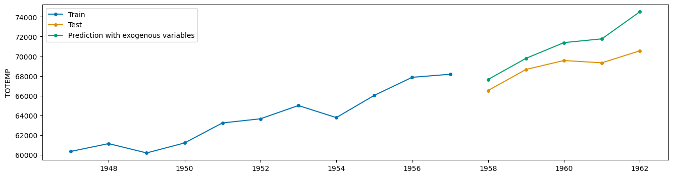

Adding exogenous data results in a much better fit on the test set! However, note that we also need the values of X when calling the predict method. If these values aren’t available, we’ll need to forecast them separately—a task that can be challenging in itself.

Pipelines

Now, let’s explore how to build more sophisticated pipelines rather than simply fitting a single model in a one-step process. This approach is similar to scikit-learn, where we can construct a pipeline that imputes missing values, standardizes numerical features, one-hot encodes categorical variables, and trains a KNeighborsRegressor at the end.

To demonstrate the power of pipelines, we’ll replace ARIMA with scikit-learn’s GradientBoostingRegressor in a recursive approach. In this setup, we train a model for one-step-ahead forecasts and then recursively call the model to generate forecasts further into the future:

from sktime.forecasting.compose import make_reduction
from sklearn.ensemble import GradientBoostingRegressor

gb_forecaster = make_reduction(GradientBoostingRegressor(), window_length=4)
gb_forecaster.fit(y_train, X_train)
y_pred = gb_forecaster.predict(fh=np.arange(1, 6), X=X_test)

plot_series(y_train, y_test, y_pred, labels=["Train", "Test", "GradientBoostingRegressor (recursive)"])

The fit is poor, but the reason for this is simple. Since this isn’t always on the radar of many data science practitioners, let me highlight a fundamental characteristic of decision tree-based algorithms:

Trees can ever output values that are higher or lower than any target that they have seen during training.

This means that using tree-based algorithms without additional adjustments will result in poor models when there’s a trend in the data, as we see here.

Dealing with trends

There are several ways to help the tree produce more meaningful values, including:

imposing a trend, or
differencing the data.

Imposing a trend means that you fit a really simple model, such as a line, through the data y and subtract it from y, giving you detrended targets y‘ = y – detrend(y). Then, you train the model on y‘. While it is easy to do with numpy or scikit-learn, it is even easier with sktime.

from sktime.transformations.series.detrend import Detrender

detrender = Detrender().fit(y_train)
detrended_y = detrender.transform(y_train)
plot_series(y_train, y_train - detrended_y, labels=["Train", "Trend"])

The actual detrended time series – subtracting the orange from the blue line – looks like this:

plot_series(detrended_y, labels=["Detrended"])

You can see that the time series no longer shows a trend, making it easier to train a tree-based model. Fortunately, you don’t need to manually detrend the time series, train a model on the detrended version, and then reintroduce the trend – sktime has you covered!

from sktime.forecasting.compose import TransformedTargetForecaster

forecaster = make_reduction(GradientBoostingRegressor(), window_length=4)
pipeline = TransformedTargetForecaster([
    ("Detrend", Detrender()),
    ("Forecast", forecaster)
])
pipeline.fit(y_train, X_train)

y_pred = pipeline.predict(fh=np.arange(1, 6), X=X_test)

plot_series(y_train, y_test, y_pred, labels=["Train", "Test", "Prediction"])

Much better! Also, note that without changing any hyperparameters, you get a linear trend. You can also change it to polynomial trends, an exponential trend, square root trend, and many more. You can even use Prophet’s trend logic using ProphetPiecewiseLinearTrendForecaster, if you like.

Note: You can also use the operator to create TransformedTargetForecaster pipelines! Just do `Detrender() forecaster` and see the magic!

As an alternative to imposing a trend, we can use differencing, which is precisely what the "I" in ARIMA represents. Essentially, instead of forecasting y directly, you forecast y.diff() in pandas logic – that is, the difference between two consecutive time series values.

from sktime.transformations.series.difference import Differencer

differencer = Differencer().fit(y_train)
detrended_y = differencer.transform(y_train)
plot_series(detrended_y, labels=["Difference"])

And with this object, you can just change the old pipeline to

pipeline = TransformedTargetForecaster([
    ("Difference", Differencer()),
    ("Forecast", forecaster)
])

if you want.

Imputation and more

Let us assume that there are missing values in the time series y, and your model does not how to handle it. You can easily impute by using skime’s versatile Imputer class.

from sktime.transformations.series.impute import Imputer

y = pd.Series([1, 2, 3, np.nan, 5])
imputer = Imputer(method="linear")
imputer.fit_transform(y)

# Output:
# 0    1.0
# 1    2.0
# 2    3.0
# 3    4.0
# 4    5.0
# dtype: float64

You can also just add it to the pipeline to let it grow even further:

pipeline = TransformedTargetForecaster([
    ("Impute", Imputer()),
    ("Difference", Differencer()),
    ("Forecast", forecaster)
])

Or we can add a log transformation as well:

from sktime.transformations.series.boxcox import LogTransformer

pipeline = TransformedTargetForecaster([
    ("Impute", Imputer()),
    ("Log", LogTransformer()),
    ("Difference", Differencer()),
    ("Forecast", forecaster)
])

There are many more transformations available, and I recommend exploring the API reference of sktime. For now, though, let’s shift our focus to hyperparameter optimization.

Hyperparameter Optimization

Alright, we’ve chained several transformations, each consisting of different objects. Each of these objects has a set of hyperparameters, and naturally, we want to find the combination that yields the best results. Let us take a look at our pipeline again:

pipeline = TransformedTargetForecaster([
    ("Impute", Imputer()),
    ("Log", LogTransformer()),
    ("Difference", Differencer()),
    ("Forecast", make_reduction(GradientBoostingRegressor()))
])

We can use pipeline.get_params() to see all the hyperparameters we can tune.

...
'Impute__forecaster': None,
'Impute__method': 'drift',
...
'Log__offset': 0,
'Log__scale': 1,
'Difference__lags': 1,
'Difference__memory': 'all',
'Difference__na_handling': 'fill_zero',
...
'Forecast__window_length': 10,
'Forecast__estimator__alpha': 0.9,
'Forecast__estimator__ccp_alpha': 0.0,
'Forecast__estimator__criterion': 'friedman_mse',
...

Just like scikit-learns GridSearchCV or RandomizedSearchCV , sktime offers [ForecastingGridSearchCV](https://www.sktime.net/en/stable/api_reference/auto_generated/sktime.forecasting.model_selection.ForecastingGridSearchCV.html) , [ForecastingRandomizedSearchCV](https://www.sktime.net/en/stable/api_reference/auto_generated/sktime.forecasting.model_selection.ForecastingRandomizedSearchCV.html) , and even [ForecastingOptunaSearchCV](https://www.sktime.net/en/stable/api_reference/auto_generated/sktime.forecasting.model_selection.ForecastingOptunaSearchCV.html) . Let us stick with the grid search version for now. Here we go:

from sktime.forecasting.model_selection import ForecastingGridSearchCV
from sktime.split import ExpandingWindowSplitter

pipeline = TransformedTargetForecaster([
    ("Impute", Imputer()),
    ("Log", LogTransformer()),
    ("Difference", Differencer()),
    ("Forecast", make_reduction(GradientBoostingRegressor()))
])

# forecast 4 steps
cv = ExpandingWindowSplitter(fh=np.arange(1, 5), initial_window=5)

grid = ForecastingGridSearchCV(
    forecaster=pipeline,
    cv=cv,
    param_grid={
        "Forecast__window_length": [1, 2, 3, 4, 5],
        "Forecast__estimator__learning_rate": [0.1, 0.05, 0.01],
        "Log__scale": [1, 2, 3],
    }
)

grid.fit(y_train, X_train)

Just like in scikit-learn, we can get the best parameters via grid.best_params_ :

{'Forecast__estimator__learning_rate': 0.01,
 'Forecast__window_length': 2,
 'Log__scale': 1}

And make predictions using

y_pred = grid.predict(fh=np.arange(1, 6), X=X_test)

plot_series(y_train, y_test, y_pred, labels=["Train", "Test", "Prediction"])

Optimize the architecture

A great feature of sktime is that we can optimize not only the hyperparameters but also the steps in the pipeline. For example, we’ve included a log transformer in the pipeline – should we keep it, or would it be better to exclude it? sktime offers the [OptionalPassthrough](https://www.sktime.net/en/latest/api_reference/auto_generated/sktime.transformations.compose.OptionalPassthrough.html) class to answer this question in an easy way:

from sktime.transformations.compose import OptionalPassthrough

pipeline = TransformedTargetForecaster([
    ("Impute", Imputer()),
    ("Log", OptionalPassthrough(LogTransformer())), # maybe use log
    ("Difference", Differencer()),
    ("Forecast", make_reduction(GradientBoostingRegressor()))
])

grid = ForecastingGridSearchCV(
    forecaster=pipeline,
    cv=cv,
    param_grid={
        "Forecast__window_length": [1, 2, 3, 4, 5],
        "Forecast__estimator__learning_rate": [0.1, 0.05, 0.01],
        "Log__passthrough": [True, False], # use log?
    }
)

grid.fit(y_train, X_train)

This can fundamentally change the architecture of the model and is a very powerful way to build your own AutoML pipeline.

Another architectural choice to consider is the order of the Log and Difference steps. It might be better to apply Difference first and then Log. However, you don’t want to manually define both versions. The problem grows as you add more steps to permute since you can reorder n steps in n! ways, which quickly becomes unmanageable. Let’s check out the Permute class!

from sktime.forecasting.compose import Permute

pipeline = TransformedTargetForecaster([
    ("Impute", Imputer()),
    ("Log", OptionalPassthrough(LogTransformer())),
    ("Difference", Differencer()),
    ("Forecast", make_reduction(GradientBoostingRegressor()))
])

permute = Permute(pipeline)

grid = ForecastingGridSearchCV(
    forecaster=permute,
    cv=cv,
    param_grid={
        "permutation": [
            ["Impute", "Log", "Difference", "Forecast"],
            ["Impute", "Difference", "Log", "Forecast"],
        ],
        "estimator__Forecast__window_length": [1, 2, 3, 4, 5],
        "estimator__Forecast__estimator__learning_rate": [0.1, 0.05, 0.01],
        "estimator__Log__passthrough": [True, False],
    }
)

grid.fit(y_train, X_train)

I think this flexibility is crazy! In our toy example, this is the result:

{'estimator__Forecast__estimator__learning_rate': 0.01,
 'estimator__Forecast__window_length': 1,
 'estimator__Log__passthrough': True,
 'permutation': ['Impute', 'Log', 'Difference', 'Forecast']}

So, essentially, our pipeline consists of imputation, differencing, and the actual forecasting step. The optimal window length is 1, and the learning rate has been reduced from the default 0.1 to 0.01.

Conclusion

sktime stands out as a powerful tool for Time Series Forecasting, offering a highly flexible and user-friendly framework that enables the seamless construction and optimization of complex pipelines. Whether you’re adding exogenous variables, experimenting with transformations like differencing and detrending, or fine-tuning hyperparameters, sktime allows you to quickly assemble the necessary components and optimize them with just a few lines of code.

Its ability to handle model architecture searches, such as testing different transformations or reordering steps, makes it a great choice for anyone looking to build sophisticated time series forecasting models.

I hope that you learned something new, interesting, and valuable today. Thanks for reading!