
INTRODUCTION
Simulation is a powerful tool in the Data Science tool box. In this article, we’ll talk about how simulation can help us make better decisions and strategies by simulating possible scenarios. One key concept we’ll explore throughout is how we can leverage machine learning models and scenario simulation to make better decisions.
The specific topics of this article are:
- Scenario simulation for Optimization
- Scenario simulation for risk management
This is the third part in multi-part series on simulation in data science. The first article covered how simulation can be used to test machine learning approaches and the second article covered using simulation to estimate the power of a designed experiment.
WHAT IS DATA SIMULATION?
The first article spends a lot more time defining simulation. To avoid redundancy, I’ll just give a quick definition here:
Data simulation is the creation of fictitious data that mimics the properties of the real-world.
Okay, with that out of the way, let’s talk about scenario simulation!
SCENARIO SIMULATION FOR OPTIMIZATION
Often, we develop machine learning models to make predictions on real data. For example, models that predict if a tumor is malignant, or if a customer is likely to default on their loan. In these cases we pass real data into our model to get predictions on real entities (patients, customers etc). When we use our machine learning models for scenario analysis, we often use simulated data to see that would happen given certain (simulated) circumstances.
For optimization, we are going to (1) simulate data that represent various strategic choices we could make, (2) use a machine learning model that was already trained on real data to make predictions on key metrics and (3) optimize our strategy based on the predicted key metrics.
Let’s look at an example of this:
Assume we are housing developers and we have already trained a model that predicts house prices. We’ll assume that this model is representative of the housing market in which we are currently developing.
Here is our house price model (made very simple to keep the example friendly):
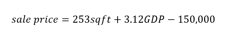
Our goal is to use our model to build the most profitable subdivision possible (predicted sale price minus cost to build). We can do this, of course, with simulation!
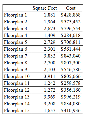
Instead of using our model to predict the sale prices of actual, existing houses, we will simulate houses based on potential floorplans and predict what the simulated houses would sell for. Let’s say we simulate the design of 15 different floorplans, their square footage and costs are shown below:
Let’s now predict the sale prices and profit of our 15 floor plans. We’ll set the GDP variable to $70,000 (approximately the current per capital GDP in the US) and generate our predictions. Note that we are using an extremely simple modeling approach, but this type of simulation is agnostic to model type.
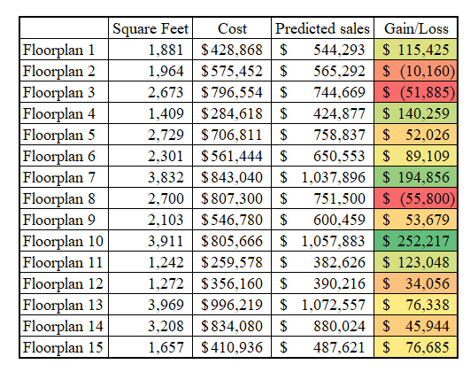
With these predictions, we have an understanding of the potential profit behind each floorplan. We now have a ton of useful information for developing an optimal strategy!
We could just pick the floorplan with the highest margin which in this case would be Floorplan 10 and build a subdivision with this design only. But that feels kind of wrong… I have two primary issues with this simple strategy: (1) I don’t know if I can trust the model’s predictions for houses in neighborhoods with just one floorplan – we would have to go back to the training data and see how far this type of strategy is away from what our model has been exposed to. For this example, let’s assume that the model has not seen monolithic neighborhoods. And, (2) this strategy assumes that the number of houses we can build in a subdivision is fixed, meaning that despite the floorplan size, we will make the same number of houses. This doesn’t seem to make much sense.
These two issues can be fixed by getting a little more fancy with our optimization. Instead of just picking the house that makes the most margin, we can create a constrained optimization problem were we select a strategy that meets requirements we establish. After deliberating with multiple groups in our company and making some additional calculations (how much lot space each floorplan uses) we’ve come up with the following requirements (aka constraints in optimization terms):
- We must have at least 6 different floorplans in our neighborhood
- We need to have at least 10 homes < 2000 sqft and 15 between 2000 sqft and 3000 sqft and 10 homes that are > 3000 sqft
- Lastly, we have 150,000 square feet of plots – each house needs 25% more square feet than the floor plan – we can’t build more houses than we have land!
Every optimization needs constraints and objectives. We have our constraints established, now it is time to get our objective set up. This is an easy one, maximize profit, or in more animated terms, MAKE MONEY!! We calculate this by multiplying the gain/loss per floor plan by the number of houses of that floorplan we will build.
Alrighty, with this all set up, we are ready to encode our objective, constraints and simulated scenario data into an optimization problem. Let’s use mixed integer linear programming as our optimization engine. Since this isn’t an article on mixed integer linear programming, I’ll provide the code below, but I’ll leave it to the reader to go through the details.
Python">import pandas as pd
import numpy as np
from pulp import *

df = pd.read_csv(csv_path)
n = len(df)

# Create a MILP problem
problem = LpProblem("Simple MILP Problem", LpMaximize)

# Define decision variables
x = LpVariable.dicts("x", range(n), lowBound=0, cat='Integer')
y = LpVariable.dicts('y', range(n), cat='Binary')

# Objective
problem += lpSum(x[i]*df['gain_loss'][i] for i in range(n))

# constraints

# limit to amount of land available
problem += lpSum(x[i]*df['square_feet'][i]*1.25 for i in range(n)) <= 150000

# requirements for diversity in home sizes
problem += lpSum(x[i]*df['small_house'][i] for i in range(n)) >= 15
problem += lpSum(x[i]*df['medium_house'][i] for i in range(n)) >= 15
problem += lpSum(x[i]*df['large_house'][i] for i in range(n)) >= 10

# Create at least 6 unique floorplans
for i in range(n):
    # if x is 0, y has to be 0
    problem += x[i] >= y[i]

# if x = 1, y coud be 0 or 1
# but because we want sum(y) to be >= 6, the optimization
# will assign y to be 1
problem += lpSum(y[i] for i in range(n)) >= 6

# solve problem
problem.solve()

# print solution
for i in range(n):
    print(f'{i + 1} : {value(x[i])}')

# print optimal profit
print("Optimal profit :", value(problem.objective))
The combination of our model, simulated data and optimization recommend we build the following 60 houses in our subdivision:
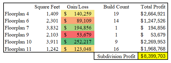
Our strategy seems to lean heavier on smaller houses because they tend to have a better margin per square foot. Because of our constraints though, we do have 6 unique floorplans in our neighborhood, with the desired spread of home sizes.
One word of caution here – with Simulation, you always must remember that garbage in = garbage out! If our model isn’t good, or our cost estimates are bad, it doesn’t matter how smart we are with our optimization; we will get bad results. It is also important to consider how the model training data compares to the simulated data. If there are data points in our simulated data that are very dissimilar from anything in the training dataset, we will likely have reason to be dubious about the predictions. For example, if the biggest house our model saw in the training dataset was 2500 sqft, we should be skeptical of predictions on 4500 sqft houses. Our model could extrapolate well to 4500 sqft, but we should look into it to make sure we are comfortable the predictions. Causality is also an implicit assumption in this approach – we are assuming that if we take certain actions, the model will predict the causal impact of those actions. If we have doubts about the causal explanatory power of the model, we my not want to take this approach until our concerns are resolved.
In conclusion, we can combine a machine learning model with simulated data to predict how our strategies may play out in the real world. We can then use an optimization technique to modify our strategy based on our specific objectives and constraints.
SCENARIO SIMULATION FOR MANAGING RISK
Let’s shift from talking about how to optimization strategies with simulation to understanding risk with simulation. In Nassim Taleb’s book ‘Fooled by Randomness,’ Taleb attributes his derivative trading success to measuring his risk by considering what could happen, rather than what has happened in the past or what is likely to happen. Simulating scenarios to understand our risk exposure helps us do just that – understand our risk stance for possible scenarios. If we just rely on historical, real world data, we may be exposing ourselves to more risk than we know because the past isn’t always representative of the future.
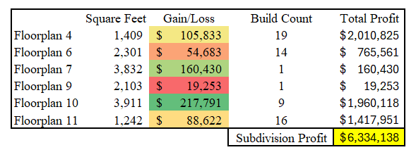
Going back to our house developer example; we now have an optimal plan to act on. Let’s say that we estimate it will take about three years to develop the neighborhood and sell all of the houses. We know that these three years will expose us to economic risk. We can use simulation to get an understanding of our risk exposure.
Let’s say that the most likely, worst case scenario is that per capita GDP drops 5% each year. This would mean that from our current level of $70,000; GDP drops 15.8% (1.05³ – 1) to $58,966. Using our model’s estimate of home sensitivity to GDP changes, our expected profit is expected to drop from $8.4mm to $6.3mm.
We need not run just one risk scenario here. We could run thousands if we wanted. In our simple approach, we only have one economic factor, but in a more nuanced approach we could have multiple both on the sales price prediction side as well as the cost side. e.g. cost of supplies/labor, interest rate changes etc. We could simulate multiple change levels on various metrics to get a better idea of our multiple risk exposures.
If in our risk simulation analysis, we see specific risk levels that are not acceptable, we can take actions to mitigate our exposure. This is the decisioning power of risk simulation. For example, if we fear that rising lumber prices expose us to excessive risk, we could buy our inventory up-front and pay to store it in a facility, or we could buy lumber futures. If we think that three years of development time exposes us to too much economic risk, we could hire more workers, rent or buy more tools and offer overtime incentives to speed up development time. These mitigating strategies will come at an extra cost, but our risk analysis (which estimates our level of exposure) paired with our risk tolerance will help us decide of the extra cost is worth the mitigation of our risk exposure.
CONCLUSION
We often want to get a better idea of what will happen in scenarios that we haven’t seen before. We can create scenarios that represent possible real-world situations to create a data-informed approach to strategic planning and risk mitigation. If we are okay with the assumptions that are associated with simulating scenarios, we can make better informed decisions to increase the probability that we reach our strategic goals.


