
The name "Monte Carlo" for the Monte Carlo methods has an origin that ties back to the famous Monte Carlo Casino located in Monaco. This name was not chosen because of any direct association with the mathematical principles behind these methods, but rather for its metaphorical connection to randomness and chance, which are central elements in both gambling and Monte Carlo simulations. In this post, we will discuss this technique and show code examples related to project management, approximating irregular areas, and gaming.
Real-world systems and processes often involve uncertain parameters and variables. With Monte Carlo methods you can explicitly model these uncertainties. Businesses can make better informed decisions by understanding the probability and impact of different risks. Besides decision support, you can use it for enhancing predictive models and/or communication.
The Basics
Imagine you have a big, mysterious jar full of different-colored marbles. There is one problem: you can’t see inside it to count how many of each color there are. You want to know which color you’re most likely to pick if you reach in the jar without looking.
You will play a game to figure this out. Instead of trying to guess or count the marbles directly (which you can’t do because you can’t see inside), you close your eyes, reach into the jar, and pull out a marble. You look at the color, write it down, and then put it back. You do this many, many times: pulling out a marble, writing down the color, and putting it back.
After you’ve done this, you look at the list. If you pulled out 100 marbles and 60 of them were red, you might start to think, "Hmm, there are probably a lot of red marbles in the jar, so I’m more likely to get a red one than any other color when I reach in."
Monte Carlo methods are all about learning something when you can’t see all the details directly. The example above is really easy: you don’t need any inputs for the model. You just start sampling to be able to draw conclusions about the outputs. Monte Carlo can be a very effective technique if you repeat your experiment for enough iterations.
Sampling, Distributions, Iterations and Convergence
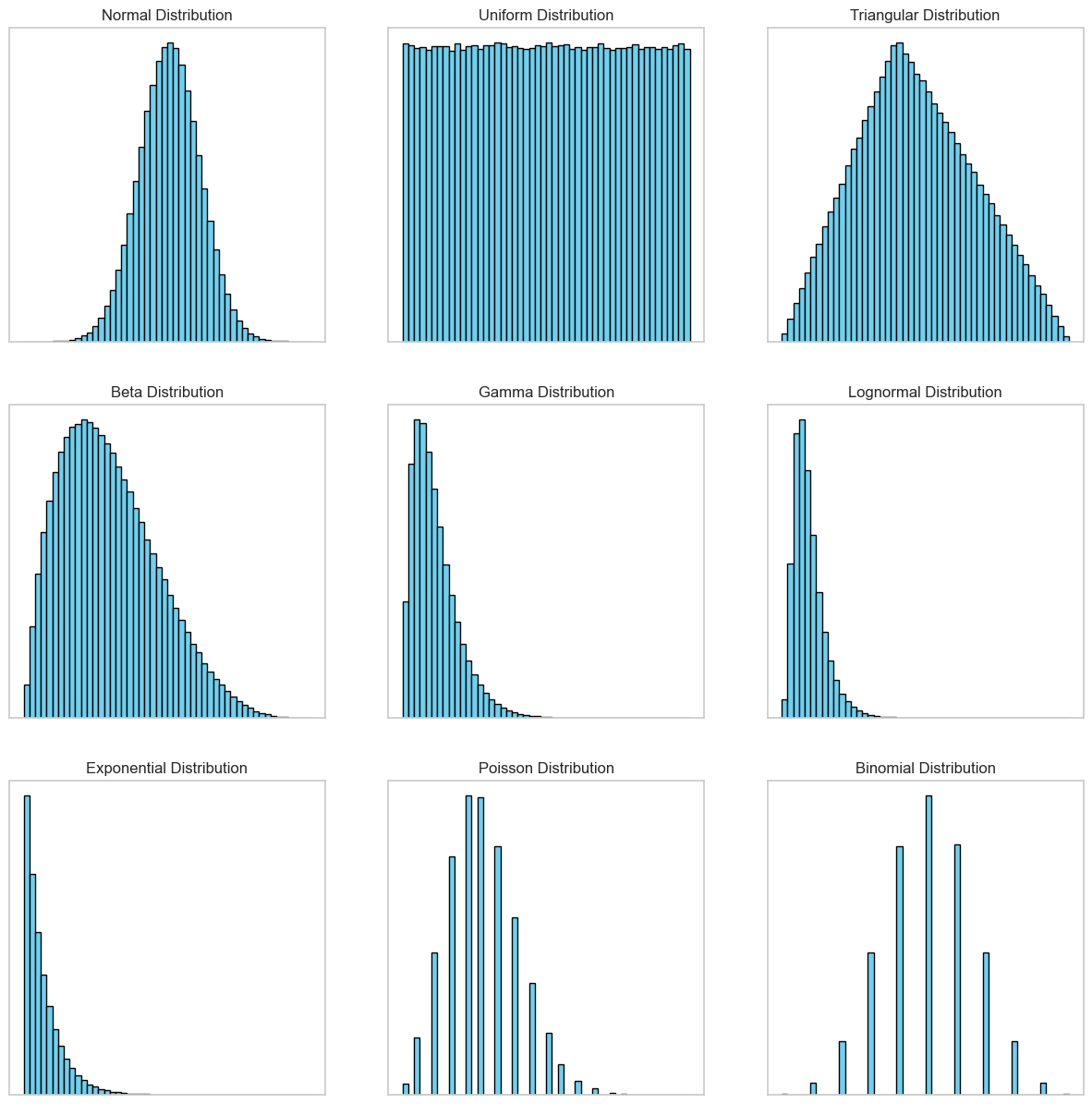
To summarize, there are three key concepts in Monte Carlo Methods. The first one is random variable sampling; for different input variables you generate values from probability distributions. The probability distributions represent the uncertainty about those variables. Common distributions include normal (Gaussian), uniform, log-normal, etc., which describe the likelihood of occurrence of different values. The third concept is iterations and convergence. Running the simulation multiple times (hundreds, thousands, or more) to ensure the results converge to a stable solution, providing a robust statistical basis for predictions.
3 Example Applications
There are many applications of Monte Carlo methods. In fact, Monte Carlo is an umbrella term: It has a broad applicability and versatility across various domains and disciplines. Monte Carlo methods contain a wide range of computational algorithms that rely on repeated random sampling to obtain numerical results. These methods are used to solve problems in fields as physics, engineering, statistics, finance, and computer science.
Let’s take a look at three common use cases and start coding! We start with Monte Carlo simulations applied in project management. After this, we will look at a completely different example: approximation of the area under (irregular) curves. We end with a technique used in game playing agents: Monte Carlo tree search.
Launch New Software
You are a project manager and responsible for the launch of a new software product, including development, testing, and market release phases, with the goal of completing the project within 6 months (180 days) from project initiation.
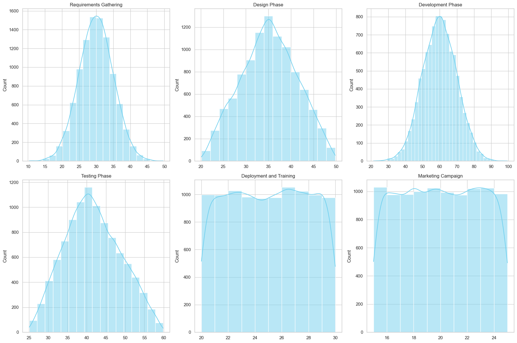
The launch is divided in six different tasks, and you discussed with involved people how long they will take approximately. This gives you the following distributions per task:
Now it’s time to run the simulation! You randomly sample 10000 times from the distributions, and add the values. Deployment and marketing can run in parallel, so you take the maximum value for those tasks. After sampling, you plot the total distribution, together with the target goal:
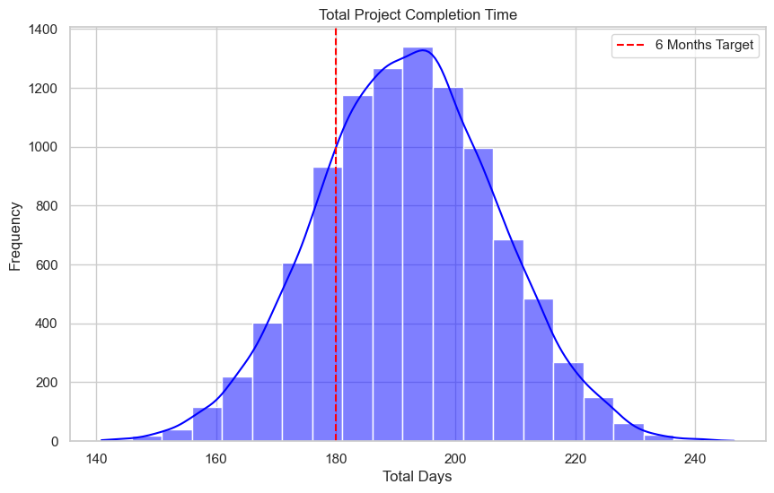
You can draw conclusions from this plot and decide if 180 days is a realistic goal for the project. Some statistics based on this simulation:
Mean Total Completion Time: 191.94 days
95% Confidence Interval: 163.04 - 221.18 days
Probability of completing the project within 6 months: 21.04%
These results can help you communicating to stakeholders. A more realistic schedule might be 200 days. Always be aware that it is hard or impossible to model all uncertainties (we’ll get back to the cons of MCS later in this post).
Code:
import numpy as np
import matplotlib.pyplot as plt
import seaborn as sns

np.random.seed(42)

n_simulations = 10000

# sample the observations from different distributions per task
requirements_distribution = np.random.normal(30, 5, n_simulations)
design_distribution = np.random.triangular(20, 35, 50, n_simulations)
development_distribution = np.random.normal(60, 10, n_simulations)
testing_distribution = np.random.triangular(25, 40, 60, n_simulations)
deployment_training_distribution = np.random.uniform(20, 30, n_simulations)
marketing_distribution = np.random.uniform(15, 25, n_simulations)

# calculate the total completion time based on the observations
total_completion_time = requirements_distribution + design_distribution + development_distribution + testing_distribution + np.maximum(deployment_training_distribution, marketing_distribution)

# plot and print results
plt.figure(figsize=(10, 6))
sns.histplot(total_completion_time, kde=True, color="blue", binwidth=5)
plt.title('Total Project Completion Time')
plt.xlabel('Total Days')
plt.ylabel('Frequency')
plt.axvline(180, color='red', linestyle='--', label='6 Months Target')
plt.legend()
plt.show()

print(f"Mean Total Completion Time: {np.mean(total_completion_time):.2f} days")
print(f"95% Confidence Interval: {np.percentile(total_completion_time, 2.5):.2f} - {np.percentile(total_completion_time, 97.5):.2f} days")
print(f"Probability of completing the project within 6 months: {np.mean(total_completion_time <= 180):.2%}")
Area under an Irregular Curve
Do you remember the rules for calculating the area under a complex curve like:

I bet you don’t! Maybe only if you are a mathematician or need to do calculations like this often. Or when you like to practice mathematical integration skills in your free time.
There are situations where it becomes impractical or impossible to calculate the area under a curve using traditional analytical mathematical methods. This can be the case in high-dimensional problems, or when the domain of integration has an irregular shape or is defined by conditions that are difficult to express mathematically. Sometimes, an approximation is good enough for the problem at hand. When it’s hard to compute the area under the curve, using Monte Carlo simulations is easy and can help to get a fast answer to the problem.
In this example we will estimate the area under the curve of the function above on the domain [0, 2π]. The curve looks like this:
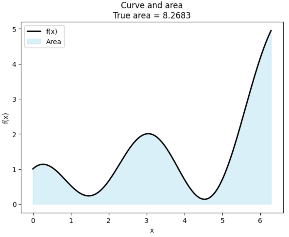
The true area is equal to 8.2683. How can we estimate the area under the curve by using Monte Carlo simulations? We take the following steps:
- We sample n random points from a uniform distribution that fall into the domain and range of the function.
- We determine the number of points that fall under the curve
y < f(x). - Here comes the trick: We multiply the domain with the range (total area of the ‘rectangle’), and multiply this with the percentage of points that falls under the curve. This gives us a good approximation.
Let’s try it in practice. We sample a number of points and calculate the estimation, as well as the error. For the error we subtract the estimation from the true area.

By adding points we get closer and closer to the actual value. Using 1 million random points, the error is only 0.0039. (This doesn’t have to be the case though, because of the randomness of Monte Carlo, but most of the times, the approximation should improve by adding points.) This approach is much simpler than mastering calculus!
Approximation of areas can be useful in more scenarios than you might think. One example is when estimating the coverage of ice sheets, forests, and bodies of water to understand climate change impacts. Or an example in astronomy: people can determine the area of celestial objects’ surfaces or the cross-sectional area of galaxies when direct measurements are not possible.
Code related to this example:
import numpy as np
import matplotlib.pyplot as plt

np.random.seed(31)

def f(x):
    return np.sin(x) + np.cos(2*x) + x**2 / 10

x_range = np.linspace(0, 2*np.pi, 10000)
true_area = np.trapz(f(x_range), x_range)

n_points_list = [100, 1000, 10000, 100000, 1000000]

fig, axs = plt.subplots(3, 2, figsize=(12, 15))
fig.subplots_adjust(hspace=0.3, wspace=0.2)

# plot 1: The curve and the actual area under the curve
axs[0, 0].plot(x_range, f(x_range), color='black', linewidth=2, label='f(x)')
axs[0, 0].fill_between(x_range, 0, f(x_range), alpha=0.3, color='skyblue', label='True Area')
axs[0, 0].set_title('Curve and areanTrue area = {:.4f}'.format(true_area))
axs[0, 0].legend()
axs[0, 0].set_xlabel('x')
axs[0, 0].set_ylabel('f(x)')

# simulation for different numbers of points
for idx, n_points in enumerate(n_points_list, start=1):
    x = np.random.uniform(0, 2*np.pi, n_points)
    y = np.random.uniform(0, max(f(x_range)), n_points)
    f_x = f(x)
    points_under_curve = y < f_x
    area_estimate = 2 * np.pi * max(f(x_range)) * np.sum(points_under_curve) / n_points

    ax = axs.flat[idx]
    ax.scatter(x[~points_under_curve], y[~points_under_curve], color='red', s=1, label='Above Curve')
    ax.scatter(x[points_under_curve], y[points_under_curve], color='blue', s=1, label='Under Curve')
    ax.plot(x_range, f(x_range), color='black', linewidth=2, label='f(x)')
    ax.set_title(f'n points = {n_points}nEstimation = {area_estimate:.4f}; Error = {abs(area_estimate - true_area):.4f}')
    ax.set_xlabel('x')
    ax.set_ylabel('y')

    if idx == 1:
        ax.legend(loc='upper left')

plt.tight_layout()
plt.show()
Monte Carlo Tree Search
When creating agents playing games, Monte Carlo tree search (MCTS) is the algorithm you will find in many solutions. In AlphaGo and AlphaZero, MCTS is combined with neural networks to determine the best next action.
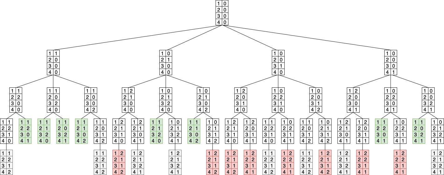
As an example, we will look at a really easy two player game. The game is called Island Conquest. There are four islands on the board, they are numbered 1–4. On each turn, a player claims one island. A player wins if he owns islands 1&2 or 1&4. Automatically, you lose if you own islands 2&3 or 3&4. If one player owns islands 1&3 and the other player 2&4, it’s a tie.

This game is super easy and would be boring to play, because the first player can always win by claiming island 1 in the first turn, and in his second turn claim island 2 or 4. For demonstrating MCTS, it’s a good game because of its simplicity. We can visualize this game as a tree:
Before we run the algorithm, let’s go over the theory. How can MCTS help us in deciding the next best action for a game? The MCTS algorithm consists of four steps:
Step 1. SelectionFirst step is to select a node (= an action) of the game tree. We start at the root node. In the beginning, we select nodes that are unvisited:

When we don’t have unvisited nodes left, we select nodes in a smarter way. Then we use the Upper Confidence bound for Trees (UCT). This is a mathematical formula that combines the number of visits with the score for the node. The upper confidence bound formula looks like this:
score / child_visits + math.sqrt(2 * math.log(parent_visits) / child_visits)If the number of visits and the corresponding scores are like this:
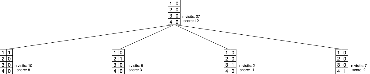
We have a total visit of 27. If we need to select our first action (from the root), the scores for the islands are:
- Island 1: 1.61
child_visits = 10;score = 8;parent_visits = 27 - Island 2: 1.28
child_visits = 8;score = 3;parent_visits = 27 - Island 3: 1.32
child_visits = 2;score = -1;parent_visits = 27 - Island 4: 1.26
child_visits = 7;score = 2;parent_visits = 27
We select the highest value, so island 1 will be selected. The upper confidence bound balances exploration and exploitation.
Note that the value for island 3 is higher than for islands 2 & 4. We didn’t explore island 3 that much yet (only 2 times), so it might be interesting to try or simulate this action a few more times to become more certain of how bad this action is.
Step 2. ExpansionDuring the expansion phase, the selected node is expanded by adding one or more child nodes to the tree, representing possible future states of the game from that point. This step only occurs if the node has unexplored actions available. The new node is added to the tree with initial scores and visit counts, ready for future simulations.

Step 3. SimulationThis step involves simulating a play-out from the state represented by the expanded node. The simulation randomly selects actions for the player until a terminal state is reached (win, loss, or draw). The outcome of this simulation provides a score that indicates the desirability of the initial move, which is used to update the game tree in the backpropagation step. In the Island Conquest game, we use 1 for a win, -1 for a loss, and 0 for a draw.

Step 4. BackpropagationIn the final step, the results from the simulation are propagated back up the tree to the root. Every node visited during the selection and expansion phases is updated to reflect the new information: the visit count is incremented, and the score for every node is adjusted based on the outcome of the simulation. This updated information influences future selection decisions, gradually improving the algorithm’s decision-making as more simulations are conducted.

Do you recognize how MCTS relates to Monte Carlo methods? Again, iterations are used to converge to the optimal action. The difference with the previous examples, is that MCTS applies the Monte Carlo philosophy to processes in environments with sequential decisions, such as board games. MCTS is not just simulating outcomes of a static set of variables (like in the project management and area under the curve examples). It is dynamically building a tree of possible future states based on the outcomes of those simulations. At each iteration, MCTS selects a path through the tree based on past results (selection), expands the tree by exploring new moves (expansion), simulates outcomes from that position (simulation), and then updates the tree with the new information (backpropagation).
After simulation, MCTS will recommend the action with the highest number of visits, because this action is the one with the highest score.
Let’s code the Island Conquest game and add MCTS to select the best possible action for every turn. The first file is islandconquest.py:
from montecarlosimulation.islandconquest.mcts import mcts

class IslandConquest:
    def __init__(self):
        """
        Initialize the game with all islands unclaimed
        0 for unclaimed, 1 for Player 1, -1 for Player 2
        Player 1 starts
        """
        self.islands = [0, 0, 0, 0]
        self.player_turn = 1

    def claim_island(self, island):
        """
        Player claims an island. Island numbers are 1-4.
        Switch turns after a valid move.
        """
        if self.islands[island-1] == 0:
            self.islands[island-1] = self.player_turn
            self.player_turn *= -1
            return True
        else:
            return False  # Island already claimed

    def check_win(self):
        """
        Mapping the win/lose/tie conditions to sums of island states.
        Calculate the sum of states for comparison with the conditions.
        Return the result of the game (winner/tie/game continues).
        """
        win_conditions = [(1, 4), (1, 2)]
        lose_conditions = [(2, 3), (3, 4)]

        island_sums = {tuple: sum(self.islands[i-1] for i in tuple) for tuple in win_conditions + lose_conditions}

        for condition in win_conditions:
            if island_sums[condition] == len(condition):
                return "Player 1 wins"
            elif island_sums[condition] == -len(condition):
                return "Player 2 wins"

        for condition in lose_conditions:
            if island_sums[condition] == len(condition):
                return "Player 2 wins"
            elif island_sums[condition] == -len(condition):
                return "Player 1 wins"

        if self.islands[0] + self.islands[2] in [-2, 2] and self.islands[1] + self.islands[3] in [-2, 2]:
            return "It's a tie"

        return "Game continues"

    def is_game_over(self):
        """
        Check if the game is over.
        """
        return self.check_win() != "Game continues"

    def current_state(self):
        """
        Print the current state of the game.
        """
        state = " ".join(["1" if x == 1 else "2" if x == -1 else "0" for x in self.islands])
        print(f"Islands: {state}")
        print(f"Player {'1' if self.player_turn == 1 else '2'}'s turn")
        print(self.check_win())

    def get_legal_moves(self):
        """
        Get the list of unclaimed islands.
        """
        return [i+1 for i, x in enumerate(self.islands) if x == 0]

    def copy(self):
        """
        Used in MCTS to copy the game state.
        """
        new_game = IslandConquest()
        new_game.islands = self.islands[:]
        new_game.player_turn = self.player_turn
        return new_game

    def get_result(self, player):
        """
        Get score of the game for the player for MCTS.
        """
        result = self.check_win()
        if result == "Player 1 wins" and player == 1 or result == "Player 2 wins" and player == -1:
            return 1
        elif result == "Player 1 wins" and player == -1 or result == "Player 2 wins" and player == 1:
            return -1
        return 0  # Tie or game continues

def play_game_with_mcts(game, mcts_iterations=1000):
    """
    Play the game with MCTS.
    Selects the best move for the current player and game state and performs it.
    """
    while not game.is_game_over():
        print("nCurrent game state:")
        game.current_state()

        best_move = mcts(game.copy(), mcts_iterations)
        print(f"Recommended move: Claim island {best_move}")

        game.claim_island(best_move)

        if game.is_game_over():
            print("nFinal game state:")
            game.current_state()
            break

if __name__=="__main__":
    game = IslandConquest()
    play_game_with_mcts(game)
This code is quite easy. First, we initialize a game with 4 unclaimed islands [0, 0, 0, 0]. Then it’s the turn for the first player, and this player can select an island. The best move for the current player is selected with Monte Carlo tree search.
The code from mcts.py is as follows:
import math
import random

class MCTSNode:
    def __init__(self, game_state, move=None, parent=None):
        """
        Initialize the node with the game state, move, and parent.
        """
        self.game_state = game_state
        self.move = move
        self.parent = parent
        self.children = []
        self.wins = 0
        self.visits = 0
        self.untried_moves = game_state.get_legal_moves()

    def select_child(self):
        """
        Select a child node with the highest UCT score.
        """
        return max(self.children, key=lambda c: c.wins / c.visits + math.sqrt(2 * math.log(self.visits) / c.visits))

    def add_child(self, move, state):
        """
        Remove the move from untried moves, create a new child node, and add it to children.
        """
        child = MCTSNode(game_state=state, move=move, parent=self)
        self.untried_moves.remove(move)
        self.children.append(child)
        return child

    def update(self, result):
        """
        Update this node - increment the visit count and update the win count based on the result.
        """
        self.visits += 1
        self.wins += result

def mcts(root_state, iterations):
    """
    MCTS algorithm. Selection, expansion, simulation, and backpropagation.
    """
    root_node = MCTSNode(game_state=root_state)

    for _ in range(iterations):
        node = root_node
        state = root_state.copy()

        # selection
        while node.untried_moves == [] and node.children != []:
            node = node.select_child()
            state.claim_island(node.move)

        # expansion
        if node.untried_moves:
            move = random.choice(node.untried_moves)
            state.claim_island(move)
            node = node.add_child(move, state)

        # simulation
        while not state.is_game_over():
            possible_moves = state.get_legal_moves()
            state.claim_island(random.choice(possible_moves))

        # backpropagation
        while node is not None:
            node.update(state.get_result(root_state.player_turn))
            node = node.parent

    for child in root_node.children:
        print(f"Move {child.move}: {child.visits} visits, {child.wins / child.visits:.2f} win rate")
    return sorted(root_node.children, key=lambda c: c.visits)[-1].move
The mcts function is called in the islandconquest.py script. Do you recognize the four steps of MCTS (selection, expansion, simulation and backpropagation)? In this code after simulation, the number of visits and scores for each move are printed. This shows the following result:
Current game state:
Islands: 0 0 0 0
Player 1's turn
Game continues
Move 1: 397 visits, 0.96 win rate
Move 2: 300 visits, 0.94 win rate
Move 4: 299 visits, 0.93 win rate
Move 3: 4 visits, -0.75 win rate
Recommended move: Claim island 1

Current game state:
Islands: 1 0 0 0
Player 2's turn
Game continues
Move 4: 486 visits, -0.02 win rate
Move 2: 503 visits, -0.02 win rate
Move 3: 11 visits, -1.00 win rate
Recommended move: Claim island 2

Current game state:
Islands: 1 2 0 0
Player 1's turn
Game continues
Move 4: 988 visits, 1.00 win rate
Move 3: 12 visits, 0.00 win rate
Recommended move: Claim island 4

Final game state:
Islands: 1 2 0 1
Player 2's turn
Player 1 wins
It found the optimal moves for the players for each turn! MCTS recommends island 1 to player 1 in the first turn, which actually is the best thing to do. The game can only result in a tie or in a win for player 1. In the second turn (player 2), it will recommend island 2 or 4, because otherwise player 1 is certain of a win (against a 50/50 chance that player 1 will select island 3 with a tie as result). You can see that the number of visits for island 2 and 4 are almost equal. In the third turn (player 1), island 4 is selected, because player 1 wins in this case.
Note: Do you see a possible improvement here? There is a big one. In step 3 of MCTS, the simulation step, we use a random play out. This approach may not accurately represent the behavior of a skilled opponent, leading to less optimal decision-making. There are ways to improve this, like training a policy network, using reinforcement learning, or an easier approach like using heuristic-based decisions. This is out of scope for this post, but if you are curious, you can find resources online explaining these techniques.
Cons
Besides all these cool applications of Monte Carlo, it’s not all sunshine. There are some cons, too. Let’s shortly go over them:
- Monte Carlo methods can be computationally expensive. Especially when the problem is complex and you want to run many simulations, you need a powerful computer (and time). This relates to the number of inputs you have: if you add more unknowns, you want to run more iterations, and the computational cost can increase exponentially.
- If the data is biased, incomplete, or inaccurate, the simulation results will be unreliable. There should be good data collection and analysis practices in place to be able to trust the results. This problem is also known as sensitivity to assumptions.
- Building a comprehensive and accurate model can be challenging, especially for systems with complex interactions and dependencies. Simplifications made to manage complexity can sometimes lead to oversights or misrepresentations of the real-world scenario. Besides building the model, interpreting the results can be hard as well! There’s a risk of misinterpretation, especially when considering the range of possible outcomes and their probabilities.
- You always need to keep in mind that simulations are not the same as precise predictions. Ensuring that the simulation has run a sufficient number of trials for the results to converge on a stable solution can be tricky. In some cases, reducing the variance of the results to achieve a desired level of precision might require an impractically large number of iterations.
Conclusion
Monte Carlo simulation is a useful technique, and can be applied in many different ways and fields. After reading this post, you learned the basics and key concepts of Monte Carlo. We went over three examples about project management, approximating areas, and Ai Gaming. Thanks for reading, and until next time!
Related
Solving Multi-Armed Bandit Problems