Handling Gaps in Time Series

Time is the most well-defined continuum in physics and, hence, in nature. It should be of no surprise, then, the importance of continuity in time series datasets – a chronological sequence of observations.

This concept alone drives the motivation behind this article. Real-world datasets are susceptible to missing values for various reasons, such as faulty sensors, failures in data ingestion, or simply the absence of information during a given time. That, however, doesn’t change the underlying nature of the data-generating process of your features.

Understanding what caused those interruptions and analyzing and handling them in a time series dataset is, therefore, paramount to any subsequent task.

---

Table of Contents

• The Goal of this Article
• Dataset Description
• Libraries and Dependencies
• Data Preprocessing
• Isolated vs. Continuous Missing Values
• Visualizing Missingness
• Subsetting Intervals for Experimentation
• Artificially Missing Data
• Imputation of Short Sequences
• Experimentation Method
• Imputation of Long Sequences
• Impact on Subsequent Analysis
• Impact on the Data Distribution
• Conclusion
• References

---

The Goal of this Article

After a comprehensive exploratory analysis of your time series, you might find that missing values are present to a considerable extent. By seeking an understanding of the nature of your data, you should be able to differentiate a gap that represents missingness from a gap that entails an actual interruption, characterizing it as an intermittent series.

This article will focus on the first scenario – analysis of missing values and methods to evaluate imputation results. While the actual techniques to perform imputation are many [1][2], I will elaborate on the approaches for gauging the quality of their results so you can assess when and where to apply them in your dataset.

Before we begin, it is worth mentioning that imputation might not always be the best route to take. Remember, in time series problems, your goal is often to craft a mathematical representation of your data-generating process (what causes the data to occur), but this concept is, by definition, a platonic ideal [3] we cannot fully reach. What missingness does is to fog that ideal, but poor imputation can drive you further away from it.

With that in mind, we will work with a hypothetical scenario where our goal is to forecast the levels of fine particulate matter in the air, also known as PM 2.5, one of the main contributors to air pollution and air quality indices. So, let’s take a look at our dataset.

---

Dataset Description

The data holds one-hour average measurements of fine particulate matter PM 2.5 (fine particles with diameters of 2.5 microns and smaller) in µg/m3 (micrograms per cubic meter) with values from January 1st, 2016, to July 3rd, 2022, across four monitoring stations in the city of Vancouver, British Columbia, Canada.

The dataset is a subset of the original one published by the British Columbia Data Catalogue [9] and contains 57,014 PM 2.5 records per station, with 4,958 missing values. It is available under the Open Government License – British Columbia [10].

import pandas as pd

master_df = pd.read_csv("data/2016_2021_master_df.csv")
master_df = pd.melt(master_df,
                    value_vars=[
                    "Vancouver_Clark_Drive_PM25",
                    "Vancouver_International_Airport_#2_PM25",
                    "North_Vancouver_Mahon_Park_PM25",
                    "North_Vancouver_Second_Narrows_PM25"
                    ],
                    ignore_index=False)
display(master_df.head())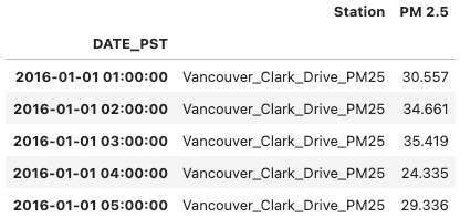

---

Libraries and Dependencies

Code examples from this article can be reproduced in any Python 3.8+ environment.

We will use Pandas and Numpy for data processing, Matplotlib and Seaborn for visualizations, and SciPy for some of our metrics. We will also use Darts, a library with a host of forecasting and anomaly detection models under a user-friendly implementation.

I will make use of some of the custom functions for visualizations introduced in my previous post. You will see them whenever I call a module named tshelpers.

---

Data Preprocessing

During preprocessing, we want to identify the missing values and quantify missingness and continuity. For that, we will start by introducing a flag isMissing.

# Dummy variable to track missing samples and missing sample length
master_df["isMissing"] = np.where(master_df["PM 2.5"].isnull(), 1, 0)
master_df.head()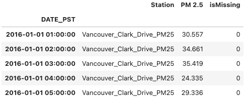

The following snippet will separate the four stations into four independent data frames.

# Isolating stations on independent data frames
datasets = {}
for station in stations:
    datasets[station] = master_df[master_df["Station"] == station]
    datasets[station] = datasets[station][["PM 2.5", "isMissing"]]
    datasets[station].reset_index(inplace=True)

Darts has a list of useful methods and functions to help quantify and locate gaps and complete sequences, such as [TimeSeries.gap](https://unit8co.github.io/darts/generated_api/darts.timeseries.html#darts.timeseries.TimeSeries.gaps) and [darts.utils.missing_values.extract_subseries](https://unit8co.github.io/darts/generated_api/darts.utils.missing_values.html?highlight=extract+subseries#darts.utils.missing_values.extract_subseries). I heavily encourage you to look into those if you are already using the library in your project, but since Darts is a fairly heavy dependency, I will define below a simple implementation that you can replicate and will suit your needs of analyzing missingness.

The following function counts the length of missing and nonmissing intervals, as well as their start and end timestamps.

def count_sequences(data, time, value):
    # Indexer for nonmissing value on data
    is_not_nan = ~data[value].isna()

    # Auxiliary indexer to group sequences
    # diff and cumsum aggregate nonmissing sequences
    group_idx = is_not_nan.diff().cumsum().fillna(0) # fillna(0) resolves cumsum's 'NaN' on idx = 0

    # Not-missing counter
    not_nan_counts = is_not_nan.groupby(group_idx).sum()

    # Instantiate sequence lengths DataFrame and retrieve position indices and time
    sequences_df = pd.Series(np.arange(len(data))).groupby(group_idx).agg(['min', 'max'])
    sequences_df['seq_start_time'] = sequences_df['min'].map(data[time])
    sequences_df['seq_end_time'] = sequences_df['max'].map(data[time])
    sequences_df['not_nan_count'] = not_nan_counts
    sequences_df['nan_count'] = (sequences_df['max'] - sequences_df['min']) - (sequences_df['not_nan_count'] - 1)

    # Assert sum of sequence lengths == total series length
    assert sum(sequences_df[['not_nan_count', 'nan_count']].sum()) == data.shape[0]

    # Tidy up
    sequences_df.rename(columns={'min': 'seq_start_idx', 'max': 'seq_end_idx'}, inplace=True)
    sequences_df.sort_values('seq_start_idx', inplace=True)
    sequences_df.reset_index(drop=True, inplace=True)

    return sequences_df

---

Isolated vs. Continuous Missing Values

From a concept well illustrated in the paper "Three-step imputation of missing values in condition monitoring datasets", we can classify missing intervals according to the length of the missing segment and the completeness of adjacent variables [5].

We will borrow from their original definition with a generalization to univariate series, where we classify a missing segment as either continuous or isolated. So, for the purposes of this article, we define:

• Isolated Missing Values (IMV): An individual observation or a sequence of observations with a length equal to or smaller than T, where data is missing for a given variable.
• Continuous Missing Values (CMV): A sequence of observations with a length larger than T, where data is missing for a given variable.

Here, T is the threshold used to classify a missing sequence as either isolated (IMV) or continuous (CMV). This definition generalizes to univariate or multivariate scenarios and offsets the decision on whether to treat complete segments (in between missing samples) as independent ones or not.

With an IMV threshold T set to 2 hours, we can now use the function count_sequences() in our dataset to measure the length of the missing segments and to classify them as individual or continuously missing.

IMV_THRESHOLD = 2 # T (in hours)

metadata = {}
for station in stations:
    metadata[station] = count_sequences(datasets[station], time='DATE_PST', value='PM 2.5')
    # Continuous Missing Values (CMV) flag
    metadata[station]['isCMV'] = (metadata[station]['nan_count'] > IMV_THRESHOLD).astype(int)
    # Isolated Missing Values (IMV) flag
    metadata[station]['isIMV'] = (metadata[station]['nan_count'].isin([i for i in range(1, IMV_THRESHOLD+1)])).astype(int)

metadata['North_Vancouver_Second_Narrows_PM25'].head()

With this metadata, we can now create a new variable, seqMissing, in the original data frames to store the length of the missing sequences and recompose our master data frame.

# Missing values metadata
for station in stations:
    for i, row in metadata[station].iterrows():
        seq_range = range(row['seq_start_idx'], row['seq_end_idx']+1)
        datasets[station].loc[seq_range, 'seqMissing'] = row['nan_count']
    datasets[station]['seqMissing'] = datasets[station]['seqMissing'].astype(int)

# Recomposing Master DataFrame
master_df = pd.concat(datasets).reset_index(level=0)

# Renaming station column
master_df["Station"] = master_df["level_0"]
master_df = master_df[["DATE_PST", "Station", "PM 2.5", "isMissing", "seqMissing"]]

# Redefining DATE_PST index
master_df.set_index("DATE_PST", inplace=True)

master_df[master_df["isMissing"] == 1].head()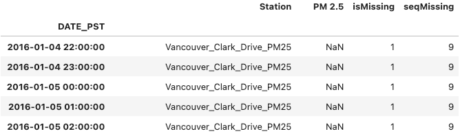

At this point, you might be asking how to define the IMV threshold T.

You can start by looking at the granularity of your dataset when it’s used for downstream Data Science or analytics tasks. If you know you are going to aggregate your data into six-hour periods, you might define T=6 and treat anything equal to or below that as individual or short sequences. We will look at the motivations for doing so in a bit.

---

Visualizing Missingness

For our first visualization, we will look at the distribution of individual versus continuous missing values in our dataset. We want to quantify them with respect to the total of missing values in each variable.

The following code will aggregate (sum) the total length of IMV and CMV gaps and plot the results in a donut chart (yes, a donut chart – please experiment with bar charts if you have more than 5 variables).

# Continuous Missing Values & Isolated Missing Values count
tot_missing = []
stations_cmv_imv = []
stations_cmv_imv_label = []

# Count of CMV and IMV intervals and percentage out of total missing
for station in stations:
    # Total missing values
    tot_missing_current = datasets[station]['isMissing'].sum()
    tot_missing.append(tot_missing_current)
    # Total Continuous Missing Value
    tot_cmv = metadata[station].loc[metadata[station]['isCMV'] == 1, 'nan_count'].sum()
    stations_cmv_imv.append(tot_cmv)
    stations_cmv_imv_label.append(f"{tot_cmv/tot_missing_current * 100:.0f}%nCMV")
    # Total Isolated Missing Value
    tot_imv = tot_missing_current - tot_cmv
    stations_cmv_imv.append(tot_imv)
    stations_cmv_imv_label.append(f"{tot_imv/tot_missing_current * 100:.0f}%nIMV")

# Stacked pie charts with IMV and CMS percentages
fig, ax = plt.subplots(figsize=(9, 9))
ax.axis("equal")
width = 0.3

# Outer pie chart (total missing values per station)
pie, texts1 = ax.pie(tot_missing, radius=1, labels=tot_missing, labeldistance=0.85,
    textprops={"fontsize": 14, "weight": "bold"})
for t in texts1:
    t.set_horizontalalignment("center")
plt.legend(pie, stations, loc=(0, -0.05))
plt.setp(pie, width=width, edgecolor="white")

# Inner pie chart (percentage of IMV and CMV out of total missing)
pie2, texts2 = ax.pie(stations_cmv_imv, radius=1 - width, labels=stations_cmv_imv_label,
    labeldistance=0.78, textprops={"weight": "bold"})
for t in texts2:
    t.set_horizontalalignment("center")
plt.setp(pie2, width=width, edgecolor="white")
plt.title("Missing Values per Station", fontsize=14, weight="bold", y=0.96)
plt.suptitle(
    "Isolated Missing Values (IMV) and Continuous Missing Values (CMV)",
    fontsize=12,
    y=0.85,
)
plt.show()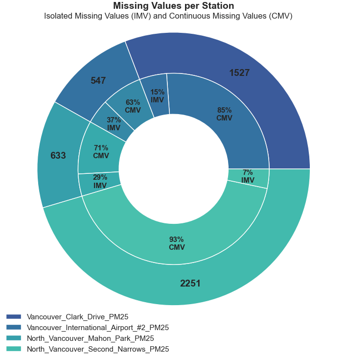

We can see that the majority of our missing values are part of a 3-hour-long sequence or higher. The plot also shows that the North Vancouver Second Narrows has the largest amount of missing values by a significant margin, and the vast majority are from long sequences.

The following visualization will give us an idea of the distribution of the sequence lengths of CMVs. We will plot a histogram and a complimentary box plot of the count of sequence lengths.

# Distribution of CMV Sequence Length
for station in stations:
    _, (ax_hist, ax_box) = plt.subplots(
        2,
        sharex=True,
        gridspec_kw={"height_ratios": (.9, .10)},
        figsize=(12,4)
    )

    plot_title = station[:-5].replace('_', ' ')
    cmv_counts = metadata[station].loc[metadata[station]['isCMV'] == 1, 'nan_count'].to_list()

    sns.histplot(x=cmv_counts, kde=True, bins=40, ax=ax_hist)
    sns.boxplot(x=cmv_counts, width=0.7, color='0.5', linecolor='#003366', flierprops={'marker': '.'}, ax=ax_box)

    ax_hist.set(title=plot_title, ylabel=f'Count of Sequences')
    ax_hist.yaxis.set_major_locator(MaxNLocator(integer=True))
    plt.suptitle('Continuous Missing Value (CMV) | Sequence Length Distribution',
                 fontweight='bold',
                 fontsize=12)
    ax_box.set(yticks=[], xlabel='Missing Values Sequence Length')
    sns.despine(ax=ax_hist)
    sns.despine(ax=ax_box, left=True)

We can see that the majority of the long sequences are approximately of length 3 to 24 hours, with some outliers beyond that range. It’s also clear why the North Vancouver Second Narrows and the Vancouver Clark Drive stations are the ones with the most missing values: They both have sequences that are 350 hours or longer.

These results hint that we can probably benefit from three different approaches to handling missing values. One imputation method for IMVs or short sequences, another (or the same) for sequences of 3 to 24 hours long, and possibly treating gaps longer than that as interrupters, where it might be better to consider in-between complete segments as independent ones, as we may lack a good model to accurately impute them.

---

Subsetting Intervals for Experimentation

To assess the quality of the imputation of short sequences, we will look for complete intervals where we can artificially create missing values to impute and evaluate the results against the real data.

First, we want an overview of where in the time span of our dataset the missing values are located and how spread out they are. We will use a heatmap for that.

from tshelpers.plot import plot_missing

plot_missing(master_df.pivot(columns="Station", values="PM 2.5"))

They are fairly spread out. With the following snippet, we will loop through each station and capture months that have no missing values. Those will be assigned as our experimentation subsets, where we will artificially gap and impute to evaluate imputation methods.

# Looking for months without missing values
months_complete = {}
for station in stations:
    months_complete[station] = []
    station_subset = master_df[master_df["Station"] == station]
    for year in range (2016, 2022):
        if year == 2022:
            range_max = 7 # Limiting upper range for 2022 as data goes up to July
        else:
            range_max = 13
        for month in range(1, range_max):
            if month == 12:
                subset = station_subset[datetime(year, month, 1, 1): datetime(year, month, 31, 23)]
            else:
                subset = station_subset[datetime(year, month, 1, 1): datetime(year, month+1, 1)]
            if subset['PM 2.5'].isna().sum() == 0:
                months_complete[station].append((month, year))

# Experimental subsets
exp_subsets = {}

for station in months_complete:
    exp_subsets[station] = {}
    for months in months_complete[station]: # Iterating on list of tuples (month, year) | (4, 2016)
        month = months[0]
        year = months[1]
        if month == 12:
            next_month = 1
            next_year = year+1
        else:
            next_month = month+1
            next_year = year
        exp_subsets[station][f'{month}-{year}'] = master_df[master_df["Station"] == station][
            datetime(year, month, 1):datetime(next_year, next_month, 1)
        ]

for station in exp_subsets:
    print(f'{station}:n {exp_subsets[station].keys()}n')

We have a total of 20 experimentation subsets, each with around 720 complete observations (30 days of 24 hours).

---

Artificially Missing Data

To programmatically create artificially missing sequences, we will define a function that takes a start and end date, the length of the desired missing interval, and the padding on where to create them (relative to the start or the end of the series).

def create_missing(
    data,
    time=None,
    value=None,
    start=None,
    end=None,
    missing_length=1,
    missing_index="end",
    padding=24,
    verbose=True,
):
    # Missing data subset
    subset_missing = subset.copy()
    subset_array = subset_missing[value].to_numpy()
    if missing_index == "end":
        missing_start = padding + missing_length
        missing_end = padding
        subset_array[-missing_start:-missing_end] = np.NaN
    elif missing_index == "start":
        missing_start = padding
        missing_end = padding + missing_length
        subset_array[missing_start:missing_end] = np.NaN
    subset_missing[value] = subset_array

    return subset, subset_missing

An artificially generated missing interval with a length of 6 hours, padded 24 hours from the end of the sequence, can be generated as follows.

from tshelpers.plot import plot_compare

station_subset = master_df[master_df["Station"] == "North_Vancouver_Mahon_Park_PM25"]

subset, subset_missing = create_missing(
    data=station_subset,
    value="PM 2.5",
    start=datetime(2019, 9, 1),
    end=datetime(2019, 9, 10),
    missing_length=6,
    padding=24,
    missing_index="end",
)

plot_compare(
    data=subset,                            # Subset to plot
    data_missing=subset_missing,            # Subset with missing values to plot
    value="PM 2.5",                         # Variable to plot from subset
    value_missing="PM 2.5",                 # Variable to plot from subset_missing
    missing_only=True,                      # Plots only the section with missing values from subset_missing
    start=datetime(2019, 9, 1),
    end=datetime(2019, 9, 10),
    fill=True,
    data_label="Artificial missing values", # Label for subset
    data_missing_label="Original data",     # Label for subset_missing
)

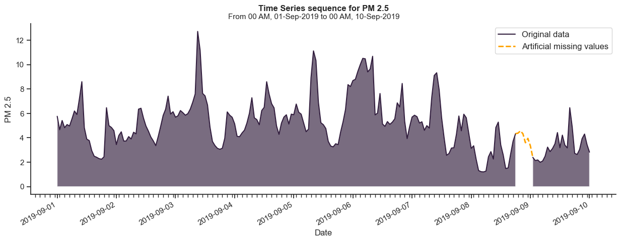
This concept will drive our experimentation method moving forward.

---

Imputation of Short Sequences

For short sequence imputation, you generally want to avoid starting with complex methods. There are several reasons for that:

1. Short sequences are, by definition, spread out and often appear in high quantities. Any imputation method that you assign to deal with those will highly benefit from being lightweight and operationally efficient.
2. In cases where the sample size of available data is limited, simple imputation methods can still provide reasonable estimates.
3. Simple imputation methods are also straightforward to interpret, as they are often derived from basic statistical properties of your data.
4. Adopt the concept of starting with a simple baseline. Only progress further on the scale of complexity if needed.

In our example, we will compare the performance of linear versus cubic interpolation for the imputation of IMVs. In simple definitions:

Linear interpolation will fit a straight line between two known points to estimate the missing values in between.

Cubic interpolation will fit a cubic polynomial function between a sequence of points to estimate the missing values in between.

The following plot illustrates the imputation with linear interpolation.

from tshelpers.metrics import rmse_score, mae_score

# Imputation with linear interpolation
subset_linear = subset.copy()
subset_linear["PM 2.5"] = (
    subset_missing["PM 2.5"].interpolate(method="linear").tolist()
)

plot_compare(
    subset_linear, subset_missing, ...,
    plot_sup_title=f"MAE: {mae_score(subset, subset_linear, value='PM 2.5', verbose=False):.4f}
| RMSE: {rmse_score(subset, subset_linear, value='PM 2.5', verbose=False):.4f}",
)

You can see that we introduced two metrics to evaluate the accuracy of the imputation:

• Mean Absolute Error (MAE): It is defined as the average of the absolute differences between generated or predicted and actual values.

• Root Mean Squared Error (RMSE): It is defined as the square root of the average of the squared differences between the generated or predicted and the actual values. It gives more weight to large errors due to its quadratic nature.

The formulas above show the two metrics as a function of a sample of n observations yi and n corresponding generated or predicted values ŷ [6][7].

While there is a multitude of accuracy metrics that can fit different purposes, we will stick with these two for our examples. You are encouraged to look for the ones that better fit the nature of your dataset.

Before we continue, a side note on Pandas’ implementation of the cubic interpolation.

---

Pandas’ default method for a cubic spline interpolation is passed to the SciPy [UnivariateSpline](https://docs.scipy.org/doc/scipy/reference/generated/scipy.interpolate.UnivariateSpline.html) function at the scipy.interpolate module and doesn’t take into account the first derivative of surrounding points to fit the curve. The following plot illustrates Pandas’ implementation of a cubic spline interpolation.

# Cubic interpolation - Pandas implementation
subset_spline = subset.copy()
subset_spline["PM 2.5"] = (
    subset_missing["PM 2.5"].interpolate(method="spline", order=3).tolist()
)

plot_compare(subset_spline, subset_missing, ...)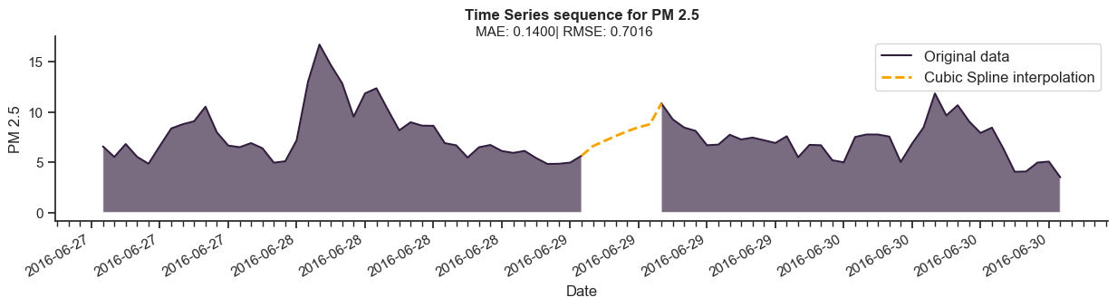

To address that, we will instead use a combination of the SciPy [splrep](https://docs.scipy.org/doc/scipy/reference/generated/scipy.interpolate.splrep.html) and [splev](https://docs.scipy.org/doc/scipy/reference/generated/scipy.interpolate.splev.html#scipy.interpolate.splev) functions. The generated results will now fit a curve that evaluates the derivative of adjacent observations.

subset_spline = subset.copy()
# Indexing missing values
missing_idx = np.where(subset_missing["PM 2.5"].isna())[0].tolist()

# Indexing boundary values at t-2, t-1, t+1, and t+2
boundary_idx = []
for idx in range(min(missing_idx)-2, max(missing_idx)+3):
    if idx not in missing_idx:
        boundary_idx.append(idx)
boundary = subset_missing["PM 2.5"][boundary_idx].tolist()

# Fitting cubic spline
cubic_spline = interpolate.splrep(x=boundary_idx, y=boundary, k=3)
imputed = interpolate.splev(missing_idx, cubic_spline)

subset_spline["PM 2.5"][missing_idx] = imputed

plot_compare(subset_spline, subset_missing, ...)

The implementation has added complexity, but the result is now as intended.

---

Experimentation Method

To accurately measure the effectiveness of an imputation method, we will iterate over:

a. The 20 experimentation subsets.

b. The length of the missing sequence (1 or 2 hours for IMVs).

c. The location of the missing sequence in the subset.

For b. and c., we will use our create_missing() function to add to the padding of the missing sequence incrementally. It will effectively slide the missing sample from right to left while covering the whole experimentation set. The image below illustrates the process.

While doing that, we will store our MAE and RMSE metrics for each iteration so we can analyze the results. For conciseness, the following snippet contains a simplified version of that implementation. At the end of the article, you can find a link to the jupyter notebook with the original code.

from darts.metrics import mae, rmse

imputation_results = {}
for station_subset in exp_subsets[station]:      
    # Generating backwards missing intervals
    paddings = [i for i in range(2, len(exp_subsets[station][station_subset]))]
    for padding in paddings:
        # Creating missing interval with length = 1 and length = 2
        for length in [1, 2]:
            subset, subset_missing = create_missing(
                data=exp_subsets[station][station_subset],
                padding=padding,
                missing_length=length
            )
            ### Cubic spline
            [...]

            # Fitting cubic spline
            cubic_spline = interpolate.splrep(x=boundary_idx, y=boundary, k=3)
            imputed = interpolate.splev(missing_idx, cubic_spline)
            subset_spline["PM 2.5"][missing_idx] = imputed

            # Evaluating cubic spline
            imputation_results[imputation_step]["RMSE_Cubic"].append(rmse(subset, subset_spline))
            imputation_results[imputation_step]["MAE_Cubic"].append(mae(subset, subset_spline))

            ### Linear interpolation
            subset_linear = subset.copy()
            subset_linear["PM 2.5"] = subset_missing["PM 2.5"].interpolate(method="linear", inplace=False).tolist()

            # Evaluating linear interpolation
            imputation_results[imputation_step]["RMSE_Linear"].append(rmse(subset, subset_linear))
            imputation_results[imputation_step]["MAE_Linear"].append(mae(subset, subset_linear))
            imputation_results[imputation_step]["Missing_Length"].append(length)

If we now plot the results, we can compare both imputation methods by looking at our accuracy metrics. For the following plot, outliers outside three standard deviations were removed for improved visualization.

The linear interpolation shows better results, and as expected, the error metrics are smaller for the imputation of a single observation (1h). To conclude with statistical significance that you have a clear winner, you might want to perform a statistical test, such as a Wilcoxon signed-rank test for paired samples (where the samples are not drawn from a normal distribution, such as in the results above).

# Linear interpolation imputation of IMVs
master_df.loc[master_df["seqMissing"] <= 2, "PM 2.5"] = master_df.loc[master_df["seqMissing"] <= 2, "PM 2.5"].interpolate()

By imputing IMVs with linear interpolation, we are now down to 4,175 missing values (from 4,958).

---

Imputation of Long Sequences

Before we begin, we can list some of the challenges associated with the imputation of longer sequences.

1. Increased Uncertainty: The greater the sequence of missing values, the greater the epistemic uncertainty of imputed values. It is not uncommon to use forecasting models to fill in long gaps in interrupted time series, and statistical models tend to rely heavily on recent observations (or lags), especially in univariate problems.
2. Impact on Data Distribution: Imputing long sequences of missing values can significantly alter the distribution of the data, and that is particularly detrimental for subsequent analyses and interpretations.
3. Evaluation of the Results: Measuring the effectiveness of the imputation method is challenging for long sequences. Traditional accuracy metrics may not fully capture the impact on temporal dynamics and trends in the data.

In simple terms, not only is it harder to impute missing values in longer sequences, but it also becomes more challenging to effectively evaluate the results.

You can probably tell that now is the time for more elaborate imputation algorithms. While model selection is not the focus of this article, you can explore the following options as your baseline:

• kNN: The k-Nearest Neighbors algorithm can be used to impute missing values using data from the k nearest neighbors that have a value for the feature.
• MICE: Short for Multivariate Imputation by Chained Equations, it is an iterative algorithm that imputes missing data through a series of predictive models.
• FFT: A Fast Fourier Transform can be used to perform forecasting by extracting the underlying periodic patterns from a time series.
• SMA: Short for Simple Moving Average, it’s an algorithm that calculates the average of a fixed finite number of previously available values to generate the subsequent set of missing ones.

And, if needed, dive into more involved architectures. Here is a list of interesting resources if you want to read more on what has been recently proposed for missing value imputation in univariate and multivariate time series:

• Fill the Gap: EDDI for Multivariate Time Series Missing Value Imputation by Microsoft researchers at Cambridge
• DeepMVI: Missing Value Imputation on Multidimensional Time Series by IIT Bombay researchers in Mumbai, India
• M-RNN: Multi Direction Recurrent Neural Networks for Missing Values Estimation by Yoon et al. 2017
• SAITS: Self-Attention-based Imputation for Time Series by Du et al. 2023 (GitHub repository here).

This time, however, we will shift our focus to the other end of the problem. Let’s introduce two additional methods to evaluate our imputation results.

1. Impact of imputation on subsequent analysis.
2. Analysis of distribution before and after imputation.

---

Impact on Subsequent Analysis

A practical way to compare two or multiple imputation methods is to assess their impact on any downstream analysis or modelling tasks.

In our example, we will assume that our goal is to forecast future levels of PM 2.5 in the city of Vancouver, and for that, we need to provide our model with data that adheres to a minimum standard of completeness and continuity. For the sake of simplicity, we will work with a naive XGBoost model.

Let’s start by defining a function to wrap the Darts TimeSeries.plot method with some extra functionalities to easily look at our error metrics, now during prediction.

from darts import TimeSeries
from darts.metrics import mae, rmse

# Auxiliar plotting function
def dart_plot(train, val, plot_title="Time Series Train/Validation Sets", pred=None, pred_label="predicted"):
    plt.figure(figsize=(12, 2.5))
    train.plot(label="training")
    val.plot(label="validation", linewidth=1, color="darkblue")
    if pred:
        pred.plot(label=pred_label, linewidth=1.5, color = "darkorange")
        plt.title(f"MAE: {mae(pred, val):.3f} | RMSE: {rmse(pred, val):.3f}", fontsize=10)
        plt.suptitle(plot_title, fontweight="bold", fontsize=11, y=1.04)
    else:
        plt.title(plot_title, fontweight="bold", fontsize=11)
    plt.legend()
    plt.xticks(fontsize=10)
    plt.yticks(fontsize=10)
    plt.ylabel("PM 2.5", fontsize=11)
    plt.xlabel("")
    sns.despine()
    plt.show()

Using the TimeSeries.split_after() method, we will split our experimentation subset into a training and a validation set.

exp_subset = master_df[master_df['Station'] == 'Vancouver_Clark_Drive_PM25']
exp_subset = exp_subset.loc[
    datetime(2019, 8, 8):datetime(2020, 9, 6),
    ['PM 2.5']
]

validation_cutoff = pd.Timestamp("2019-11-29 19:00:00")
exp_subset_series = TimeSeries.from_dataframe(exp_subset)
train, val = exp_subset_series.split_after(validation_cutoff)

We also need to define which lags (or past observations) the model will use for prediction. For our example, due to the seasonal nature of our data, we will use multiples of 6 lags across the last 48 hours.

max_lag = 48
step = 6

[-i for i in range(step, max_lag+step, step)]

This gives us a list of [-6, -12, -18, -24, -30, -36, -42, -48] lags to be used for prediction.

We will use a probabilistic version of the XGBoost model by defining the parameter likelihood='poisson' to draw a prediction interval. Below is a sample forecast of 24 time steps (in hours), sampled 200 times from the model.

from darts.models import XGBModel

model = XGBModel(
    lags=lags,
    output_chunk_length=2,
    likelihood='poisson',
    random_state=42
)
model.fit(train)
pred = model.predict(n=24, num_samples=200)
dart_plot(train[-48:], val[:24], pred=pred)

We’ve got a period of relatively high PM 2.5 index to predict in our example (the mean PM 2.5 measurement is 6.2 µg/m3 across all four stations in the dataset). The model anticipates the increase in the index by the afternoon of November 30th but with high uncertainty, with the prediction interval shooting all the way up to 80 µg/m3.

Shifting our focus back to the original problem, we want to see the impact that imputed missing values in our training set have on the forecasted period. For that, we will define a function that evaluates how many points in the validation set fall within the 95% prediction interval.

def evaluate_prediction_interval(pred: TimeSeries,
                                 val: TimeSeries,
                                 lower_quantile: float=0.05,
                                 upper_quantile: float=0.95) -> np.ndarray:
    # Lower and Upper prediction interval series
    lower_bound = pred.quantile_timeseries(lower_quantile).all_values().flatten()
    upper_bound = pred.quantile_timeseries(upper_quantile).all_values().flatten()

    # Validation set
    val_flatten = val.all_values().flatten()

    # Accuracy vector
    accuracy_vector = np.logical_and(
        val_flatten >= lower_bound,
        val_flatten <= upper_bound
    )

    return accuracy_vector

This function returns a boolean array that we can use to determine the coverage of our prediction interval.

coverage = sum(evaluate_prediction_interval(pred, val[:24]))/len(pred)
print(f'Prediction Interval coverage: {coverage*100:.2f} %')

The metric tells us that 83.33% of the validation set is within our prediction interval. In the following examples, we will remove 12 hours from our training set and see how two imputation methods, a linear interpolation and an FFT recomposition, impact these results.

_, train_missing = create_missing(
        data=train,
        value="PM 2.5",
        missing_length=12,
        padding=12,
        missing_index="end",
)

# Linear interpolation
train_linear = train_missing.copy()
train_linear["PM 2.5"] = (train_missing["PM 2.5"].interpolate(method="linear").tolist())

plot_compare(train_linear[-72:], train[-72:])

# FFT imputation
train = TimeSeries.from_dataframe(train)
fft_model = FFT(nr_freqs_to_keep=None)
fft_model.fit(train[:(-24)]) # -(missing_length + padding)
fft_pred = fft_model.predict((12)) # predicting n = missing_length steps
train_fft = train_missing.pd_dataframe().copy()
fft_pred_df = fft_pred.pd_dataframe().copy()
train_fft.loc[train_fft["PM 2.5"].isna()] = fft_pred_df[["PM 2.5"]]

plot_compare(train_fft[-72:], train[-72:])

As we can see, the FFT imputation is not able to capture the peak in PM 2.5 in the artificially generated missing interval. So, let’s see how both imputation methods impact the prediction with our XGBoost model.

model = XGBModel(
    lags=lags,
    output_chunk_length=2,
    likelihood='poisson',
    random_state=42
)
model.fit(train_linear)
pred = model.predict(n=24, num_samples=200)
dart_plot(train_linear[-48:], val[:24], pred=pred)

coverage = sum(evaluate_prediction_interval(pred, val[:24]))/len(pred)
print(f'Prediction Interval coverage: {coverage*100:.2f} %')

model = XGBModel(
    lags=lags,
    output_chunk_length=2,
    likelihood='poisson',
    random_state=42
)
model.fit(train_fft)
pred = model.predict(n=24, num_samples=200)
dart_plot(train_fft[-48:], val[:24], pred=pred)

coverage = sum(evaluate_prediction_interval(pred, val[:24]))/len(pred)
print(f'Prediction Interval coverage: {coverage*100:.2f} %')

The coverage of the prediction interval clearly indicates that the poor performance of the FFT imputation is affecting our forecast.

---

Impact on the Data Distribution

Another way to assess whether the stretched imputation of a large gap is within reasonable values is to look at the data distribution before and after the imputation.

One way to evaluate that is by simply plotting a histogram of our original training set and comparing it to the imputed one. That, however, doesn’t give us a quantitative metric to determine how well the new values fit into the distribution of the original data.

To solve that, we can borrow from the concept of relative entropy measurement between two probability distributions, also known as Kullback-Leibler (KL) divergence. It is a type of statistical distance that measures how one probability distribution Q differs from another reference P distribution [8]. It is calculated by the formula:

We can use the KL divergence to compare the distribution of our training sets before and after imputation. So, let’s see what it tells us about the example from the last section.

# KL Divergence
from scipy.special import rel_entr

KL_Div_linear = sum(rel_entr(train[-48:].values(), train_linear[-48:].values()))
KL_Div_fft = sum(rel_entr(train[-48:].values(), train_fft_imputed[-48:].values()))

fig, axes = plt.subplots(1, 2, figsize=(10, 5), sharey=True)

sns.histplot(train[-48:].pd_dataframe(), x="PM 2.5", label="OriginalnData", kde=True, color="navy", bins=10, ax=axes[0])
sns.histplot(train_linear[-48:].pd_dataframe(), x="PM 2.5", label="LinearnInterpolation", kde=True, color="orange", bins=10,  ax=axes[0])
sns.histplot(train[-48:].pd_dataframe(), x="PM 2.5", label="OriginalnData", kde=True, color="navy", bins=10, ax=axes[1])
sns.histplot(train_fft_imputed[-48:].pd_dataframe(), x="PM 2.5", label="FFTnImputation", kde=True, color="orange", bins=10,  ax=axes[1])
plt.suptitle(f"PM 2.5 Distribution", fontsize=13, fontweight="bold", y=0.95)
axes[0].set(title=f"KL Divergence Linear: {KL_Div_linear[0]:.3f}")
axes[0].legend()
axes[1].set(title=f"KL Divergence FFT: {KL_Div_fft[0]:.3f}")
axes[1].legend()
plt.xlabel("PM 2.5")
plt.tight_layout()
sns.despine()
plt.show()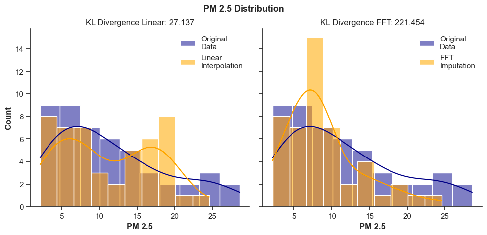

A higher KL Divergence means that the distribution diverges further from the original training data. So, from the results above, we can clearly see how it penalizes the bad imputation of the FFT model.

---

Conclusion

When faced with a time series dataset with missing values, it is easy to focus and dive in head first into model selection. As we have seen in the latest sections, the possibilities are vast and the amount of options grows as I write.

But as important as the imputation algorithm, it is fundamental to:

1. Perform a thorough analysis of your missing values. You might often benefit from splitting your imputation methods into distinct steps that fit intervals of different sizes.
2. Define a proper evaluation strategy. Assessing imputation performance must not rely only on accuracy metrics. You can always benefit from looking at the distribution of your data and the impact on downstream tasks.

You can find a jupyter notebook with details of the implementation shown in this article here.

Enjoyed this Story?

You can follow me here on Medium for more articles about data science, Machine Learning, visualization, and data analytics.

You can also find me on LinkedIn and on X, where I share shorter versions of these contents.

Get an email whenever Erich Silva publishes.

---

References

[1] Fang, C., & Wang, C. (2020). Time Series Data Imputation: A Survey on Deep Learning Approaches. ArXiv. /abs/2011.11347

[2] Anna Richter , Jyotirmaya Ijaradar , Ulf Wetzker , et al. Multivariate Time Series Imputation: A Survey on available Methods with a Focus on hybrid GANs. TechRxiv. November 21, 2022.

[3] ReneBt (https://stats.stackexchange.com/users/195935/renebt), What does a data-generating process (DGP) actually mean?, URL (version: 2020–08–28): https://stats.stackexchange.com/q/451230

[4] Services, Ministry of Citizens’. "The BC Data Catalogue." Province of British Columbia. Province of British Columbia, February 2, 2022. https://www2.gov.bc.ca/gov/content/data/bc-data-catalogue

[5] Liu, H., Wang, Y., & Chen, W. (2020). Three-step imputation of missing values in condition monitoring datasets. IET Generation, Transmission & Distribution, 14(16). https://doi.org/https://doi.org/10.1049/iet-gtd.2019.1446

[6] Wikimedia Foundation. (2023, November 25). Mean absolute error. Wikipedia. https://en.wikipedia.org/wiki/Mean_absolute_error

[7] Wikimedia Foundation. (2024, January 8). Root-mean-square deviation. Wikipedia. https://en.wikipedia.org/wiki/Root-mean-square_deviation

[8] Wikimedia Foundation. (2024, January 10). Kullback–Leibler divergence. Wikipedia. https://en.wikipedia.org/wiki/Kullback%E2%80%93Leibler_divergence

[9] Services, Ministry of Citizens’. "The BC Data Catalogue." Province of British Columbia. Province of British Columbia, February 2, 2022. https://www2.gov.bc.ca/gov/content/data/bc-data-catalogue

[10] Engagement, G. C. and P. (2024, January 30). Open government licence – british columbia. Province of British Columbia. https://www2.gov.bc.ca/gov/content/data/open-data/open-government-licence-bc

Unless otherwise noted, all images are by the author.