Towards Deep Learning for Relational Databases

towards Deep Relational Learning

We got very much used now to read about deep learning, making the headlines with various breakthroughs in research domains ranging from vision and image generation to game playing. However, most of deep learning methods are still quite distant from everyday business practices. A lot of companies successfully transformed into the data-driven era, collecting large amounts of valuable data as part of their processes. And while most of such companies do use various data analytics tools to extract insights from these data, only rarely do we see engagement of actual deep learning methods, unless they directly match the business domain (e.g., image data processing companies).

In this article, we argue that one of the core reasons for this lack of neural networks in business practice is the gap in the learning representation assumed by virtually all the Deep Learning models and the, by far most common, data storage representation used in everyday practice – relational databases.

To close this gap, we introduce a principled approach of generalizing state-of-the-art deep learning models for direct application on databases through integration with the formal principles underlying every relational database engine. We then instantiate this approach with a practical tutorial in a Python framework designed for easy implementation of existing and novel deep relational models for learning directly with databases.

Learning Representations

While there are countless statistical and machine learning models present off-the-shelf within hundreds of frameworks and libraries, one aspect about them remains basically universal – the learning data representation. No matter whether you are fine with basic logistic regression, want to step-up to tree ensembles, or create advanced deep learning models, no matter whether you choose to pay for proprietary solutions with SPSS, or program from scratch with Tensorflow, you are always expected to provide the data in the form of numeric tensors, i.e. n-dimensional arrays of numbers.

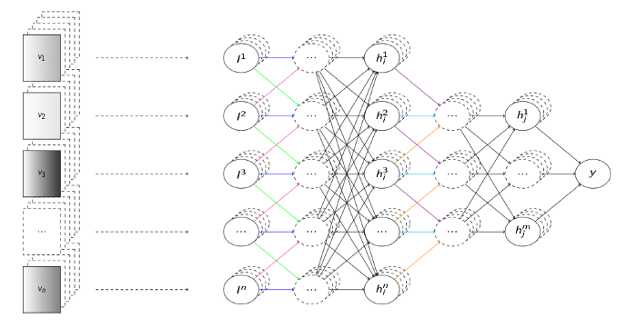
This comes down to the traditional learning representation of feature vectors, forming the 1-dimensional case of these tensors. Historically, no matter the learning domain, all the classic machine learning models have been designed for feature vector inputs. Here you, as a domain expert, were expected to design characteristic features of your problem in scope, assemble a number of these into a vector, and perform repeated measurements of these feature vectors to create a sufficiently large training dataset. At least that was the case until the deep learning revolution came with its representation learning paradigm, which largely removed the need for the manual design of these input features, and replaced them with larger amounts of raw data instead.

• Here the idea is that the characteristic features emerge as part of the training process itself, commonly referred to as embeddings, i.e. numeric vector representations of objects embedded into a shared n-dimensional space.

However, while celebrating this step-up from feature crafting to neural architecture crafting, it might come unnoticed that the learning representation is actually still exactly the same – numeric vectors/tensors.¹

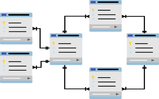
This is not a coincidence as there are understandable reasons behind using this form of representation for learning – partly historical, partly mathematical, and partly practical (as explained in our previous article). However, this representation is by far not as universal as it might seem to machine learning practitioners. Just look around to see how the actual real-world data look like. It is not stored in numeric vectors or tensors, but in the interlinked structures of internet pages, social networks, knowledge graphs, biological, chemical, and engineering databases, etc. These are inherently relational data that are naturally stored in their structured form of graphs, hypergraphs, and, most generally, relational databases.

Now comes the obvious question – can’t we just turn these data structures into our feature vectors (numeric tensors), and directly utilize all the nice machine learning (deep learning) that we have already developed? And while this is very tempting, there are deep underlying problems with such an approach:

1) There is obviously just no way to turn an unbound relational data structure into the common fixed-size numeric tensor without loss of information.

• By the way, a tensor is an example of a relational data structure, too (it is a grid). If the example tensor is bigger than the expected model input, we have a big problem.

2) Even if we limit ourselves to bounded representations, there is a principled problem with ambiguity of such a transformation, stemming from the inherent symmetries of the relational structures.

• Assume just the graph data structure here for simplicity. Should there be an unambiguous, injective mapping between graphs and tensors, it would just trivially solve the (hard) graph isomorphism problem.

And even if you just don’t care about the loss of information and ambiguity, both leading to severe learning inefficiencies, and decide to turn the structures into the vectors anyway, you are back to feature crafting.

• there are actually many ways for doing that, such as aggregating (counting) out objects, relations, various patterns (subgraphs) and their statistics, commonly referred to as "propositionalization" (relational feature extraction), which can also be automated.

And while useful in practice, such relational feature crafting is arguably uncool as it is incompatible with the core idea of deep (representation) learning. So, can we somehow resolve this to apply deep learning to relational structures in a principled manner? This will, unpopularly, require solutions beyond the common deep learning remedies (such as throwing bigger data onto a bigger Transformer…).

Relational Representations

What are these relational representations, anyway, and why should we need them? Let’s start with the popular feature vector representation of learning data. Such data can also be thought of as a table, where each column corresponds to a feature (or target label), and each row corresponds to a single independent learning example – a feature vector. Hence, we can easily store feature vectors in any database with just a single table. Now assume that the feature vectors are not so independent anymore, and one element in one feature vector can actually represent the same object as another element in another feature vector. This is actually very common in practice, where people use such vectors to represent overlapping sequences in time-series data, words in a sentence, items in a shopping cart, or figures on a chessboard. In all such cases, the elements in these vectors can no longer be thought of as simple independent values, but references to the underlying objects which then carry the actual features. Hence, conceptually, we end up with 2 tables now, where the first one contains the, possibly repeated, object references into the second table, which carries the (unique) objects’ feature values.

• In formal database terminology, a table is also called a relation, as it relates the objects from the columns together.

Arguably, such vectors can also be thought of as sequences of the objects. This then allows us to think about generalization into vectors of varying lengths, which can be taken advantage of with sequence models such as recurrent neural networks. Further, such sequences can start branching, leading to the tree data representation, such as sentence parse tree data, and models such as recursive neural networks. Finally, we can generalize to generic graph-structured data, representing anything from molecules to social networks, which is the representation at which the modern graph neural networks operate.

• this is also the representation at which the popular Transformers effectively operate – these, although technically taking sequences at input, turn them internally into fully connected graphs by assuming all pair-wise element relations within the (self-)attention module.

Do all these models also fall under the relational (database) formalism? Of course they do – these are all examples of binary relation processing. This means that to store a graph (sequence, tree) in a database, it suffices to create a single table with two columns corresponding to the two nodes connected by an edge. Each graph is then simply a collection of such edges, each stored in a separate row. For variously labeled graphs, the associated attributes can then again be efficiently stored in a separately referenced table, as before.

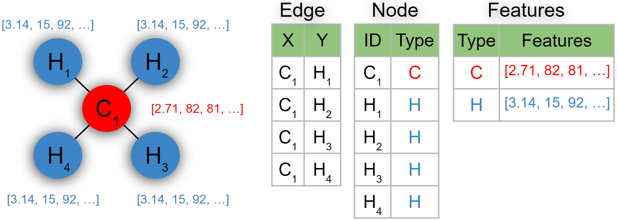
Note that this illustrates another important generalization introduced by the relational representations, which is that a single row no longer corresponds to a single learning instance, as we can generally have examples of varying sizes and structures, spanning multiple tables through the object references. Finally, databases are not limited to the binary relations, since a database table can easily relate more than two objects (i.e., each table is a hypergraph).

Hopefully, this makes it clear that we can easily capture all the commonly used learning representations in a relational database (but not vice versa). This makes the underlying relational logic (algebra) formalism a very potent candidate for an ideal learning representation!

• note that all the languages for structured data storage and manipulation used in practice, such as SQL and ERM, follow from the relational algebra and logic.

However, while these are standard formalisms for data operations as well as business practices, they might, unfortunately, seem far removed from the representations usable in machine learning. Nevertheless, that only applies to the common machine learning…

Relational Machine Learning

For decades, far from the spotlights of the deep learning mainstream, researchers have actually been developing learning approaches based directly in the aforementioned relational logic formalism within a niche subfield known as relational learning, outlined in a previous article. Briefly, relational learning methods, such as Inductive Logic Programming (ILP), provide a very elegant way for learning highly expressive, efficient and interpretable models. This approach truly demonstrates the generality of the relational logic formalism, which here is used not only to capture the data and learning representations, but also the models themselves, while providing an effective way to incorporate background knowledge and domain symmetries.

The resulting models naturally allow for learning from databases, where different samples consist of different types and numbers of objects, with each object being characterized by a different set of attributes, spanning across multiple interlinked tables. While this would be a nightmare scenario for any classic machine learning algorithm, it is the standard for ILP.

However, besides these favorable characteristics, these approaches also lack severely in robustness, accuracy, and scaling – aspects in which the deep learning recently dominated the whole field.

Deep Relational Learning

Naturally, the complementary strengths of the relational and deep learning paradigms call for their integration, which we refer to as "Deep Relational Learning", the general principles of which we detailed in a previous article, followed by a practical framework called PyNeuraLogic, described in the **** subsequent one.

Briefly, the key essence was to take the lifted modeling paradigm, known from relational graphical models in _Statistical Relational Learning_, and extrapolate it into the deep learning setting. In other words, this meant to introduce a new, declarative, relational logic-based "templating" language that is differentiable, thus allowing to encode deep learning models, while keeping the expressiveness of the relational logic representations and inference.

And since this surely sounds very abstract, let us take a look at something familiar – Graph Neural Networks (GNNs), which can be seen as a simple example of a Deep Relational Learning model.

• GNNs are currently one of the hottest topics in deep learning, underlying many of the recent breakthroughs in drug discovery, protein folding, and science in general. Additionally, Transformers are actually a type of GNNs, too.

Example: Graph Neural Networks

So now we already know that a graph is just a set of edges (edge(X,Y)) between some nodes (X and Y). The essence of any GNN model is then to simply propagate and aggregate representations of nodes from their neighbors (aka "message passing"). In the relational logic terms, this message passing rule can actually be put into a logical rule as:

message2(X) <= message1(Y), edge(X, Y)

which can be intuitively read as:

To compute representation ‘message2‘ of an object X, aggregate representation ‘message1‘ of all such objects Y, where ‘edge‘ holds between the X and Y.

Now let us take a closer look at what this means from the formal, declarative, relational logic perspective. The logical predicates "message2"_, "message1"_ and "edge" here represent names of relations, while the logical variables "X" and "Y" represent references to some objects. Both "message1" and "message2" are unary relations, commonly representing some attributes of an object, while "edge" is a binary relation, relating two objects together, i.e. connecting two nodes in a graph with an edge here. The "<=" operator is an implication, commonly written right-to-left in logic programming, meaning that the (truth) value of the right part ("body" of the rule) implies the left part ("head" of the rule). Finally, the comma "," represents a conjunction, meaning that the relations "message1(Y)" and "edge(X, Y)" must hold at the same time, i.e. for the same objects Y and X.

And now let’s take a look at the same principle from the database (SQL) perspective, which reveals what is happening under the hood from a bit more familiar, practical point of view. We already know that the logical relations correspond to tables in a database. Similarly, the logical variables correspond to their columns. The table in the rule’s "head" (left side) is to be implied (<=), i.e. created, through evaluation of the "body" of the rule (right side). The logical conjunction "," in the body then corresponds to a join between the respective tables, with constraints following the respective variable binding. For instance, here we want to join tables "message1" and "edge" on their respective column Y, and store the column X (projection) of the result into a new table called "message2". And while there might be multiple objects for which such a constraint holds, i.e. multiple Ys with an "edge" from a particular X, we will also need to group by X, while aggregating the attributes of the neighboring Y’s (we can also aggregate values from the binary "edge" too). Thus, the GNN rule actually also corresponds to a simple SQL query, which can be read as:

Join tables ‘message1’ and ‘edge’ on the column Y, group by X, and aggregate the resulting values into a new table ‘message2’.

If you just stop and think about this, this is exactly the "message-passing" graph propagation/aggregation rule underlying all the GNN models.

• there you typically see the representation of the table "edge" in the form of an adjacency matrix (instead of this adjacency list/table), and the table "message1" as the feature/embedding matrix of the nodes. The propagation step, i.e. the join and aggregation here, can then be expressed through matrix multiplication of the two.³

Now we just need to add some learnable parameters to this computation pattern, in order to make it a statistical Machine Learning model in the common sense. This is done by simply associating each relation in the rule with a learnable (tensor) weight.

Finally, we "just" need to make these logical rules, i.e. the SQL queries, differentiable in order to learn those associated weights efficiently. While we will not go into details about the semantics of the differentiable interpretation of this language, it is outlined in a previous article and described further in close detail in this dissertation. Briefly, each procedural step of the underlying query evaluation represents some operation in the respective computation graph, which we then backpropagate through in a manner similar to classic deep learning models.

To summarize, we’ve just shown how to represent a classic deep-learning GNN model as a simple, parameterized SQL query. Isn’t that beautifully weird? And while this may sound like some abstract concept that you might read in a research paper, but doesn’t really work in practice, let us now make it clear that we mean this very literally with the following practical tutorial on creating an in-database GNN.

Creating in-database GNNs

Let us now switch to a practical framework that instantiates all the aforementioned Deep Relational Learning principles we have discussed so far. It is called PyNeuraLogic and you can read more about it in a previous article. Here, let us jump straight into one of its (recent) modules dealing with the mapping between the relational logic representations, used internally in the framework, and the relational databases.

As opposed to the common tensor-centric deep learning frameworks, PyNeuraLogic builds everything upon the logical relations. And since relations (tables) are first-class citizens in the framework, there is no need for any ad-hoc (problematic) tensor transformation, making its inter-operation with relational databases extremely natural. Particularly, the PyNeuraLogic framework is equipped with a set of tools for direct relation-table data mapping, training contemporary deep relational models directly upon it, and even exporting into plain SQL code, so that you can evaluate your trained models directly in your database!

Example Database

First, let us introduce the data we will work with in this simple demonstration. Our example database here contains structured information about molecules. Each molecule has some attributes, and is formed by a varying number of atoms. Atoms also have some attributes, and can form attributed bonds with other atoms. Therefore, our database consists of three tables – "molecule", "atom", and "bond".

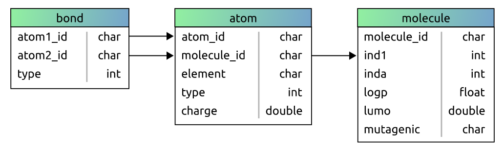
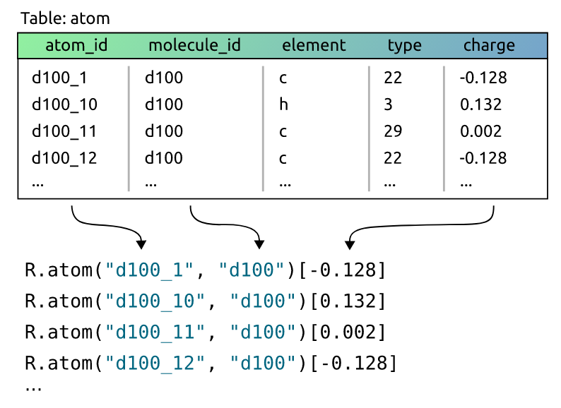
In this scenario, our task is to determine the mutagenicity of a molecule, which is one of the most commonly used benchmarks in relational learning and GNNs. Hence, our target label will be the "mutagenic" field in the "molecule" table. Now, these 3 tables will naturally correspond to 3 relations in the PyNeuraLogic framework already. However, we can also customize this mapping a bit. For example, we might want to map each row of the "atom" table to a relation "R.atom" with merely the "atom_id" and "molecule_id" columns as the relation’s terms, and the "charge" column as the relation’s value.

• Note that assigning values to relations (relational facts) is beyond the standard relational logic formalism, where the value is limited to either True (present) or False (not present). Relaxing to a full range of (tensor) values is what enables PyNeuraLogic to integrate the deep learning functionality into the relational logic principles.

Note that this mapping is very flexible. We could of course take "charge" just as another term (the value would then just default to True or "1"), include also the "element" and "type" columns, or we could even split the table into multiple newly defined relations.

To instantiate this relation-table mapping, we then create an instance of a "DBSource" object with "relation name", "table name", and "column names" (that will be mapped to terms) as arguments. To keep it simple, we will utilize only data from the "bond" and "atom" tables here:

from neuralogic.dataset.db import DBSource, DBDataset

atoms = DBSource("atom", "atom", ["atom_id", "molecule_id"], 
                  value_column="charge")
bonds = DBSource("bond", "bond", ["atom1_id", "atom2_id", "type"],
                  default_value=1)

Next, for supervised training, we will also need query labels – i.e. simply the "mutagenic" field within the "molecule" table here. Since these are textual labels, we will just want to turn them into numeric values for standard (crossentropy) error optimization, which can be customized as well:

queries = DBSource("mutagenic", "molecule", ["molecule_id"], 
                    value_column="mutagenic",
                    value_mapper=lambda value: 1 if value == "yes" else 0
)

Finally, we just put these mappings together and establish a database connection through some compatible database driver (such as psycopg2 or MariaDB) to create a relational logic_dataset:

import psycopg2

with psycopg2.connect(**connection_config) as connection:
    dataset = DBDataset(connection, [bonds, atoms], queries)
    logic_dataset = dataset.to_dataset()

• Note there is no preprocessing hidden here, such as some transformation into tensors, necessary for the common frameworks. This is just a very direct mapping between tables and relations, which can then be learned from directly with proper deep relational models.

Example GNN Model Template

The relational dataset is ready; let us now take a look at defining the learning template. We deliberately avoid the common term learning "model", since a template can be seen as a high-level blueprint for constructing such models instead. That is, a single relational template may correspond to multiple models, i.e. computational graphs, which will be automatically tailored w.r.t. each example structure and its target query here.

• This allows for universal treatment of the problem of varying size and structure of the input data. For instance, a single example molecule here corresponds nicely to a single row in the "molecule" table, which could be directly used as input for standard models (trees, SVMs, neural networks, etc.). But the same molecule also spans across a varying number of rows in the "atom" and "bond" tables, which is deeply problematic for the standard models, as explained in a previous article. Hence the generalization of "models" to "templates".

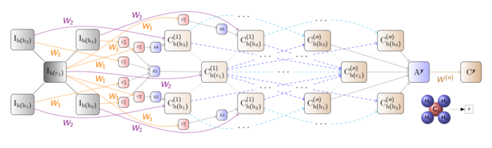
The template we will define here firstly calculates embeddings for each type of a chemical bond (bond type is just its multiplicity in the range(1,8)). Then we add two message-passing rules (GNN layers), similar to those described earlier in this article, for propagating the atom and bond representations throughout the molecule. Finally, the template defines a "readout" rule that aggregates representations of all nodes from all the layers into a single "mutagenic" value, which is passed into a sigmoid function and matched against the binary target query label for the mutagenicity classification.

• this is a classic GNN model architecture with skip connections and additional edge (bond) embedding propagation, similar to GIN.

from neuralogic.core import Template, R, V, Transformation

template = Template()

template += [R.bond_embed(bond_type)[1,] for bond_type in range(1, 8)]

template += R.layer1(V.A)[1,] <= (
    R.atom(V.N, V.M)[1,], R.bond_embed(V.B)[1,], R._bond(V.N, V.A, V.B) )

template += R.layer2(V.A)[1,] <= (
    R.layer1(V.N)[1,], R.bond_embed(V.B)[1,], R._bond(V.N, V.A, V.B) )

template += (R.mutagenic(V.M)[1,] <= (
    R.layer1(V.A)[1,], R.layer2(V.A)[1,], R.atom(V.A, V.M)[1,] )
) | [Transformation.IDENTITY]

template += R.mutagenic / 1 | [Transformation.SIGMOID]

• PyNeuraLogic overloads Python with logic programming so that you can write neural model templates through parameterized rules like this. R stands for relation generator, V for variable, [1,] are the associated weight dimensions (i.e. scalars here), and <= connects the relational pattern from the body (right side) to the rule’s head (left side). Additional information such as non-default activation functions can be appended. If this makes no sense, please see the documentation for a quick starter.

Finally, we can build and train our model by passing this template into an "evaluator", which looks very similar to classic deep learning frameworks:

from neuralogic.nn import get_evaluator
from neuralogic.core import Settings, Optimizer
from neuralogic.nn.init import Glorot
from neuralogic.nn.loss import CrossEntropy
from neuralogic.optim import Adam

settings = Settings(
    optimizer=Adam(), epochs=2000, initializer=Glorot(), 
    error_function=CrossEntropy(with_logits=False)
)

neuralogic_evaluator = get_evaluator(template, settings)
built_dataset = neuralogic_evaluator.build_dataset(logic_dataset)

for epoch, (total_loss, seen_instances)  
    in enumerate(neuralogic_evaluator.train(built_dataset)):

    print(f"Epoch {epoch}, total loss: {total_loss}, 
            average loss {total_loss / seen_instances}")

Translating Neural Models to SQL

Additionally, with just a few lines of code, the model that we have just built and trained can be turned into (Postgres) SQL code. By doing so, you can evaluate the model on further data directly in your database server without installing NeuraLogic or even Python. Just plain PostgreSQL will do!

All we have to do is to create a converter that takes our model, "table mappings", and settings. Table mappings are similar to the "DBSource", described earlier, for mapping between relations and tables:

from neuralogic.db import PostgresConverter, TableMapping

convertor = PostgresConverter(
    neuralogic_evaluator.model,
    [
        TableMapping("_bond", "bond", ["atom1_id", "atom2_id", "type"]),
        TableMapping("atom", "atom", ["atom_id", "molecule_id"], 
                      value_column="charge")
    ],
    settings,
)

After an initial setup (please see the documentation), you can install your actual model as SQL code that can be retrieved by simply calling "to_sql":

sql = convertor.to_sql()

You are now set and ready to evaluate your trained model directly in the database without the data ever leaving it. For each learning representation, there will be a corresponding function in the "neuralogic" namespace. Let’s say we would want to evaluate our model on a molecule with an id "d150" – this is now as simple as making one SELECT statement:

SELECT * FROM neuralogic.mutagenic('d150');

Similarly, we can ask for all inferrable substitutions and their values by using "NULL" as a placeholder, e.g. asking for all the molecule predictions here:

SELECT * FROM neuralogic.mutagenic(NULL);

And in exactly the same way, we can even inspect internal representations of the model! For example, we can query the value of the chemical atom with id __ "d15_11" from the _first laye_r:

SELECT * FROM neuralogic.layer1('d15_11');

Conclusion

In summary, we used the PyNeuraLogic framework to declare from scratch a simple GNN model variant that works natively on relational databases with multiple interlinked tables. Additionally, we even exported the model into plain SQL so that it can be further evaluated anytime directly in your database engine, without any external library.

This demonstrates that existing modern deep learning principles for structured data can be effectively captured under the (database) representation formalism of (weighted) relational logic. However, obviously, the point of using the vastly more expressive, differentiable relational logic formalism is that it allows you to do much more than simple graph propagation through binary relations (GNNs).

Just directly extrapolating from the GNN example, there is nothing stopping you from extending to higher-arity relations, different propagation patterns joining across more tables, and combining these into hierarchical logic (SQL) programs in novel ways. Thus, no need to wait for the next year’s NeurIPS to introduce another round of novel "deep hyper-graph", "deep meta-graph", "deep reasoning", "deep logic", and other deep relational learning ideas – you can already start simply declaring these on your own in PyNeuraLogic right now.

Just $pip install neuralogic and start putting these model ideas into practice, or reach out to us if interested!

---

1. in this article we do not make much distinctions between vector and tensor representations, since you can always translate one to another, knowing the dimensionalities, which are always known/fixed in standard deep learning models.
2. of course traversing graphs natively with recursive self-joins in a relational database is not the most efficient way to process these structures (there are, e.g., specialized graph databases for that). However, NeuraLogic uses a custom, highly efficient CSP-based relational (logic) inference engine that is very suitable for complex structured queries over highly interconnected structures.
3. this matrix form is arguably very elegant, too, but that only applies for the basic GCN models. Moving to the more expressive GNN models exploiting, e.g., the graph (sub-)structures and more advanced propagation schemes, the matrix-algebraic formalism gets messy very fast, while the relational logic formalism stays exactly the same.

---

_The author is grateful to Lukas Zahradnik for proofreading these posts, creating the tutorial, and developing PyNeuraLogic._