LinkedIn's response to Prophet - Silverkite and Greykite

Notes from Industry

Back in 2017, Facebook released its Prophet model which had quite a big impact on the domain of time series forecasting. Many businesses started using it and testing out its functionalities as it provided quite good results out of the box. Fast forward a few years and now LinkedIn enters the field with its own algorithm called Silverkite and a Python library named greykite, which is – I quote – a flexible, intuitive, and fast forecasting library.

In this article, I will provide an overview of the new algorithm and library. I will also try to point out some similarities and differences between Silverkite and Prophet. As this is a very fresh library, released in May 2021, there is still much more to explore and learn about using it in practice. I must say I am really looking forward to it and this article is just the start!

Silverkite

As you can imagine knowing LinkedIn’s business, while creating the Silverkite algorithm they had a few things in mind that the model should cope with: it must work well on time series with potentially time-varying trends, seasonality, repeated events/holidays, short-range effects, etc. You probably recognize a few common elements with Prophet, but we will get back to that.

Given what I described above and knowing that the forecasts will be run at scale, the authors focused on the following properties while developing Silverkite:

flexibility— according to the paper [1], the model handles "time series regressors for trend, seasonality, holidays, changepoints, and autoregression". And it is up to the users to choose which of the available components they do need and fit the selected ML model. Naturally, good default values and models are provided, so it is easy to use Silverkite out of the box.
interpretability— it is not only the performance that matters, often what is just as important (or even more when it comes to convincing the stakeholders) is the explainability of the approach. That is why Silverkite provides "exploratory plots, templates for tuning, and explainable forecasts with clear assumptions" (see [1]).
speed— the last one is connected to the forecasting at scale part. That is why Silvekite allows for fast prototyping (using the available templates) and deploying the created model at scale.

With Silverkite, there is no single equation to present as the model. That is why I will use the diagram from the original paper to provide an overview of the architecture and its components.

Silverkite's architecture diagram. Source: [1] — Silverkite’s architecture diagram. Source: [1]

Let’s start with the description of the colors. The green objects are the inputs to the model – the time series, potential event data, already identified anomalous data, potential future regressors (that we know will play a role in the forecast), auto-regressive components, and the changepoints. As with Prophet, we can either provide the changepoints ourselves – based on domain knowledge – or let Silverkite figure those out by itself. There is a nicely described algorithm for changepoint identification, but for that, I refer you to the original paper.

Orange indicates the outputs of the model – forecasts together with prediction intervals and diagnostics (accuracy metrics, visualizations, and summaries).

Lastly, the blue color stands for the computation steps of the algorithm. When inspecting the rectangles, we can also see some numbers there, which indicate the phases of the computations:

phase 1 – the conditional mean model – used for predicting the metric of interest,
phase 2 – the volatility model – a separate model is fitted to the residuals.

The authors state in [2] that such a choice of architecture helps with the flexibility and speed, as the integrated models are "susceptible to poor tractability (convergence issues for parameter estimates) or divergence issues in the simulated future values (predictions)".

Let’s dive a bit deeper into each of the sub-phases of computation:

1.a – this part handles extracting potential features from timestamps (hour, day of the week, month, year, etc.), as well as the events data such as holidays.
1.b – in this part, the features are transformed to appropriate basis functions (for example, Fourier series terms). The idea behind this transformation is to have features in a space that can be used in additive models for the sake of interpretability.
1.c – changepoint detection for both trend and seasonality over time.
1.d – in the last step of this phase, an appropriate ML model is fitted to the features from steps 1.b and 1.c. The authors suggest using regularized models such as Ridge or Lasso for this step.

In the second phase, a conditional variance model can be fitted to the residuals, so that the volatility is a function of the specified factors, such as the day of the week.

I would say that this would be enough introduction. At this point, I also wanted to mention two notable features that attracted my attention:

by providing external variables we can also include domain experts’ opinions. Imagine that for some kind of a forecast the experts already have quite a good idea of how it will evolve over time. We can use such an external variable to try to help the model.
including the time before/after holidays/special days. This is a feature that can come in handy in many forecasting tasks, but the first that comes to mind is a retail forecast, such as sales. In such a scenario, days around certain holidays (think Christmas) have a much different dynamic than normal days throughout the year. To make it even more interesting, the days before might have a very different pattern than the days after!

Lastly, I wanted to get back to the comparison of the two models – Silverkite and Prophet. To do so, I will show one table from Silverkite’s documentation, which presents a high-level comparison of the models.

The main differences are in the models that are being fitted and speed. For a detailed comparison of the customizable options of the two models, please see another table here.

So when to use Silverkite and when Prophet? As always, it depends. In general, the authors say to use the one that works better for your use case. Fair enough. But they also provide further hints. If you are a fan of the Bayesian approach or need logistic growth with changing capacity over time, use Prophet. On the other hand, if you want to forecast a quantile (instead of the mean) or need a fast model, then use Silverkite.

That would be it for the introduction. Let’s see how to use the model in practice!

`greykite` in practice

For this article, I will use the adapted code from the official documentation. In the example, we will use the Peyton Manning wiki pageview data – the same dataset that is used in Prophet’s documentation. We start by importing the libraries.

I might be nitpicking, but the imports are not very straightforward and will require getting used to. Then, we load the data using the DataLoader class.

If you have ever used Prophet, I am sure you recognize the familiar structure of the dataframe. As we will now see, greykite is more flexible in terms of naming. As the next step, we define some meta-information about the dataset.

Now it is time to instantiate the model. First, we create an object of the Forecaster class and then create the configuration. We specify that we want to use Silverkite (we can easily plug in Prophet here for a comparison, as it is also available in greykite). The idea behind model templates is that they provide default model parameters and allow us to customize them in a more organized way. In this case, we are interested in a forecast horizon of 365 days and 95% confidence intervals. Lastly, we run the forecast using the specified configuration and our data.

By default, greykite will use 3-fold time series cross-validation (based on an expanding window). As we have the fitted model, we will now sequentially inspect a few elements of interest. First, we can plot the original time series.

https://gist.github.com/erykml/9293e2428815faf4f511af9e90be38bd

Then, we inspect the results of the cross-validation using the following snippet.

By default, the run_forecast_config method provides complete historical evaluation. There are two kinds of outputs, the one from cross-validation splits stored in grid_search and the results of the holdout test set stored in backtest.

In the table below, we can see the MAPE (Mean Absolute Percentage Error) across the 3 splits. In the snippet, we specified cv_report_metrics=None to make the output more concise. You can remove it to see all available metrics and columns.

Now, let’s take a look at the backtest, so the holdout test set.

What we can see in the plot is the combination of the fitted values (until the end of 2015) and then the forecasts on the test set (never seen during training), which is the entire 2016. We also see the 95% confidence interval we requested in the model’s template. We can use the following snippet to see some evaluation metrics on both the train and test sets.

The table below contains only the selected metrics, the original output is much more detailed and you can see it in the Notebook (link at the end of the article).

Lastly, we can inspect the actual forecasts. Remember, we have already inspected the fitted values and the performance of the test set. But as we specified in the configuration a while back, we were interested in forecasting 1 year ahead, so for 2017.

This was already quite a lot, but please bear with me for a while longer. We have obtained the forecast, which is great, however, we still need to cover a few things to complete the basic introduction. The next item on the list is some helpful diagnostics.

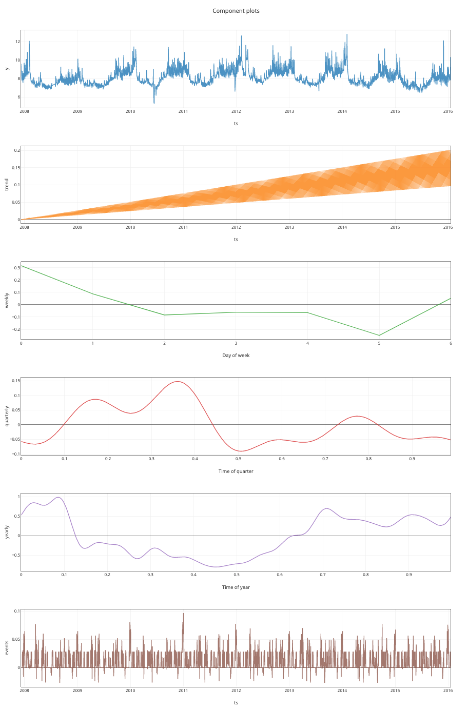
Just as in Prophet, we can see the decomposed time series. We just need to run the following:

We can see the series, together with the trend, weekly, quarterly and yearly components. Lastly, we see the impact of events. For a list of what Silverkite takes as defaults for events, please take a look here.

Then, we can also view the model’s summary to inspect the coefficients of the model. This output will be familiar to anyone who worked with statsmodels before. We use the [-1] notation to extract the estimator from the underlying scikit-learn Pipeline.

As before, I truncated the list to save some space. That is why only a few values are visible. The summary is already helpful, as we see the number of features used, the kind of estimator (Ridge), and the selected hyperparameter value.

And as the very last step, we will create some new predictions. Similarly to Prophet, we create a new future dataframe and then use the predict method of the fitted model.

You might wonder why we see predictions for 2016 here and not 2017. That is because the default settings of the make_future_dataframe method create those 4 observations just after the end of the training data. And as we have seen before, we used 2016 as a holdout test set, so it was not used for training. Remember that when creating the future dataframe, you need to pass all the extra regressors that might be necessary to make the forecast. And that was not the case for this simple example.

For a deep-dive, be sure to check out the documentation and other quickstart examples.

Takeaways

Silverkite is LinkedIn’s new time series forecasting model, similar to some extent to Facebook’s Prophet.
the model was created to deal with time series with potentially time-varying trends, seasonality, repeated events/holidays, short-range effects, etc.
greykite is the library providing a unified framework for time series forecasting and it includes Silverkite and Prophet.

You can find the code used for this article on my GitHub. Also, any constructive feedback is welcome. You can reach out to me on Twitter or in the comments.

If you liked this article, you might also be interested in one of the following:

Facebook’s Prophet + Deep Learning = NeuralProphet

The best book to start learning about time series forecasting

Introduction to hierarchical time series forecasting – part II