Why start using sktime for forecasting?

Hands-on Tutorials

The role of forecasting

One of the challenges faced by business owners is predicting future market conditions. Forecasts help to make informed decisions and form realistic expectations of results. This demand for predictions leads to the ongoing development of Forecasting tools. They enable predicting future events by grasping useful information from past observations. Some of the recent forecasting frameworks include Facebook’s Prophet, Uber’s Orbit, or Linkedin’s Greykite. Yet, most of the Python forecasting packages focus on a specific model family, e.g. generalized additive models or statistical models. Sktime aims to fill the gap between those forecasting tools.

What is sktime?

Sktime is an open-source toolbox for time series modeling. It combines functionalities spread across many Python libraries. It also adds its own unique features for forecasting. It allows us to train, fine-tune and evaluate models for time series. It is compatible with scikit-learn. The framework also enables, e.g. time series classification, feature extraction and time series clustering. For a complete list of features check out sktime’s documentation. This article focuses on forecasting and how sktime makes the whole process easier. It is a practical walk-through of sktime’s functionalities for forecasting. But first, let’s take a quick look at the data used in this article.

Data overview

All code examples are based on a public dataset from the statsmodels library. It contains USA quarterly macroeconomic data between 1959 and 2009. A full description of the dataset is available here. We will focus on predicting real gross domestic product (realgdp).

*Macroeconomic indicators over time. Image by author*

Sktime puts certain constraints on the data structure used to store the time series. You can find the macroeconomic data import and transformations below.

But to the point…

Why use sktime for forecasting?

1) It combines many forecasting tools under a unified API

Sktime brings together functionalities from many forecasting libraries. Upon that, it provides a unified API, compatible with scikit-learn.

What are the advantages of a unified API in that case? Here are some of the main reasons:

It allows users to easily implement, analyze and compare new models.
It helps to avoid confusion in choosing an appropriate algorithm thanks to a clear classification of forecasters.
It makes the workflow readable and understandable as all forecasters share a common interface. They are implemented in separate classes, as in other toolboxes, including scikit-learn.
It enables altering forecasters in a workflow. This saves us from adjusting the structure of our code each time we change our model.

Sktime’s forecasters share crucial scikit-learn’s methods, such as fit() and predict(). The code below shows a basic forecasting workflow.

Output:
2002Q2    11477.868

The code above generates a one-step-ahead forecast. That is why we assigned one to the forecasting horizon. Let’s now focus on different possibilities of specifying the horizon.

The forecasting horizon can be an array of relative or absolute values. Absolute values are specific data points for which we want to generate forecasts. Relative values include a list of steps for which predictions will be made. The relative forecasting horizon is especially useful if we make rolling predictions using the _updatepredict() method. It saves us from updating the absolute horizon each time we generate predictions. The relative horizon stays constant as we add new data.

We can also convert relative horizons to absolute horizons and vice versa. Converting from absolute to relative values is especially worth mentioning. It does not simply produce a list of step numbers. Those values relate to the last date of the training series. This means that if the values are negative, they are in-sample forecasts. This feature is important as forecasters can fit different parameters to each step. The code below shows the differences between forecasting horizons.

Output:
Absolute FH: ForecastingHorizon(['2002Q2', '2002Q3', '2002Q4', '2003Q1', '2003Q2', '2003Q3','2003Q4', '2004Q1', '2004Q2', '2004Q3', '2004Q4', '2005Q1', '2005Q2', '2005Q3', '2005Q4', '2006Q1', '2006Q2', '2006Q3', '2006Q4', '2007Q1', '2007Q2', '2007Q3', '2007Q4', '2008Q1', '2008Q2', '2008Q3', '2008Q4', '2009Q1', '2009Q2', '2009Q3'], dtype='period[Q-DEC]', name='date', is_relative=False)

Relative FH ahead: [1, 2, 3, 4, 5, 6, 7, 8, 9, 10, 11, 12, 13, 14, 15, 16, 17, 18, 19, 20, 21, 22, 23, 24, 25, 26, 27, 28, 29, 30]

Relative FH in-sample: [-29, -28, -27, -26, -25, -24, -23, -22, -21, -20, -19, -18, -17, -16, -15, -14, -13, -12, -11, -10, -9, -8, -7, -6, -5, -4, -3, -2, -1, 0]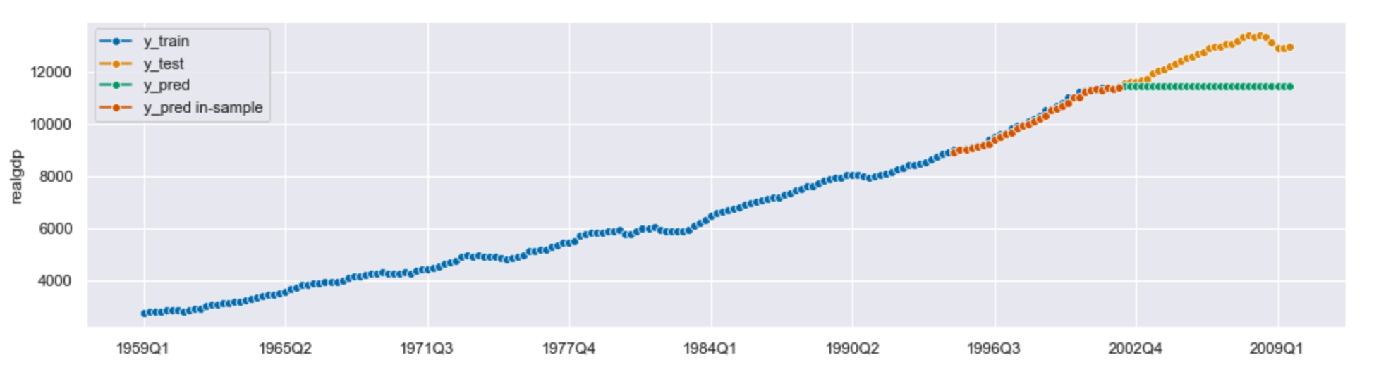

*Comparison of forecasting horizons. Image by author*

Let’s now dive into some common interface functionalities that sktime provides. First of all, the process of specifying and training the model is split into separate steps. We specify the forecaster’s parameters before fitting the model. In the case of univariate time series, the fit() method takes in the training series. For some forecasters, e.g. DirectTabularRegressionForecaster or DirectTimeSeriesRegressionForecaster, it also takes in the forecasting horizon. For others, the forecasting horizon can be interchangeably passed in the predict() method. Below is an example of forecasting a univariate time series using AutoARIMA.

*Forecasting with univariate series. Image by author*

Sktime also allows forecasting with exogenous variables. With multivariate exogenous time series, the range of fitting parameters is broader. It includes both a training series and a data frame with exogenous variables. As with univariate time series, some forecasters require the forecasting horizon in the parameters. In the code below we’re forecasting values of realgdp, using lagged values of an exogenous variable – realinv.

Forecasting with an exogenous variable. Image by author.

Apart from fitting, sktime also enables updating forecasters with new data. This allows us to automatically update the cutoff for predictions, so we don’t need to change the horizon ourselves each time we add new data. The cutoff is set to the last data point in the new training series. This method allows us to update the fitted parameters of the forecaster.

A common interface applies to all families of models. Sktime includes a wide range of easy-to-use, well-integrated forecasters. Here is a list of forecasters currently implemented in sktime:

Holt-Winter’s Exponential Smoothing, Theta forecaster, and ETS (from statsmodels),
ARIMA and AutoARIMA (from pmdarima),
BATS and TBATS (from tbats),
Prophet forecaster (from fbprophet),
Polynomial Trend forecaster,
Croston’s method.

Sktime also allows the use of scikit-learn’s Machine Learning models for modeling time series. This leads us to the next great advantage of sktime.

2) It provides machine learning models adjusted for time series problems

As I mentioned earlier, sktime’s API is compatible with scikit-learn. This implies the possibility to adapt lots of scikit-learn’s functionalities. Sktime allows us to solve forecasting problems using machine learning models from scikit-learn.

But why can’t we use standard regression models available in scikit-learn? In fact, we can, but the process requires lots of handwritten code and is prone to mistakes. The main reason is the conceptual difference between those two learning tasks.

In tabular regression, we have two types of variables – target and feature __ variables. We predict the target variable based on feature variables. In other words, the model learns from a set of columns to predict the value of a different column. The rows are interchangeable as they are independent of each other.

In forecasting, we only need to have a __ single variable. We predict its future values based on its past values. That is – the model predicts new rows of the same column. The rows are not interchangeable as future values depend on past values. So even if we forecast with an exogenous variable it is still not a regression problem.

*Tabular regression vs forecasting. Image by author*

The difference between those two problems is pretty clear. But what are the risks of using regression models in forecasting problems? Here are some of the reasons why:

It generates problems with evaluating forecasting models. Using scikit-learn’s train test split can cause data leakage. In forecasting problems, rows depend on each other so we cannot shuffle them at random.
The process of transforming data for forecasting is prone to mistakes. In forecasting tasks, we often aggregate data from multiple data points or create lagged variables. This transformation requires lots of hand-written code.
The time-series parameters are hard to tune. Values like lag size or window length are not exposed as parameters of scikit-learn’s estimators. This means we need to write extra code to adjust them to fit our problem.
Generating multi-step predictions is tricky. Let’s consider generating forecasts for the next 14 days. Regressors from scikit-learn make 14 predictions based on the last observed value. That is not what we want to do. We expect our forecaster to update the last known value every time we generate a forecast. That is, each prediction should be based on a different data point.

Sktime allows the use of regression models as components within forecasters. That is possible due to the reduction.

Reduction is the concept of using an algorithm to solve a learning task that it was not designed for. It is the process of going from a complex learning task to a simpler one.

We can use reduction to transform a forecasting task into a tabular regression problem. This means we can solve a forecasting task using scikit-learn’s estimators, e.g. Random Forest.

The key steps that take place in the reduction process are:

Using a sliding window approach to split the training set into fixed-length windows.

To give you an example – if the window length is equal to 11, the process looks as follows: the 1st window contains data from days 0–10 (where days 0–9 become feature variables and day 10 becomes the target variable). The 2nd window contains data from days 1–11 (where days 1–10 become feature variables and day 11 becomes the target variable), etc.

Arranging those windows on top of each other. This gives us data in tabular form, with clear distinction between feature and target variables.
Using one of the following strategies – recursive, direct, or multi-output, for generating forecasts.

_Using a regression model for a forecasting task. Image from sktime's documentation._ — _Using a regression model for a forecasting task. Image from sktime’s documentation._

Let’s now look at some code, performing forecasting with a regressor component.

In our example sktime’s method _makereduction() creates a forecaster based on reduction, using a scikit-learn’s model. It takes in a regressor, the name of the strategy for forecasting and window length. It outputs a forecaster which can be fitted like any other forecaster. You can alternatively use the DirectTabularRegressionForecaster object to reduce a forecasting problem to a tabular regression task. However, this forecaster uses the direct strategy for reduction.

What’s worth mentioning, the reduction’s parameters can be tuned like any other hyperparameter. This brings us to the next advantage of sktime, which is evaluating models.

3) It enables quick and painless evaluation of forecasting models

Evaluating forecasting models is not a simple task. It requires tracking different metrics than in the case of standard regression problems. They are not always easy to implement, e.g. mean absolute scaled error (MASE). Validation of those models can also be tricky, as we cannot divide our data into random subsets. And finally, tuning forecasters’ parameters, e.g. window length requires lots of hand-written code and is error-prone. Sktime addresses those three main issues connected to evaluating forecasting models.

Sktime allows the evaluation of forecasters through back-testing. This process includes splitting our data into temporal training and test sets. What’s important, the test set contains data points ahead of the training set. The rest of the process is what we know from scikit-learn. We generate predictions on the test set and calculate the metric. Then we compare forecasts with the actual values.

Sktime provides several performance metrics specific for forecasting models. They include, e.g. mean absolute scaled error (MASE) or mean absolute percentage error (MAPE). You can invoke those metrics in two ways – either by calling a function, or a class. Using the class interface provides more flexibility. It allows you e.g. to change the parameters of the metrics. What is great, sktime also offers easy implementation of custom scorers using the _make_forecastingscorer() function. An example of defining a custom metric and evaluating a model is shown below.

Output:
custom MAPE: 0.05751249071487726
custom MAPE per row:
date
2002Q2    0.001020
2002Q3    0.003918
2002Q4    0.002054
2003Q1    0.004020
2003Q2    0.009772
Freq: Q-DEC, dtype: float64

Evaluating our model on the test set is not always an optimal solution. Is there a way to adapt cross-validation for forecasting problems? The answer is yes, and sktime does it pretty well. It provides time-based cross-validation.

It enables the usage of two methods of splitting the data for cross-validation. They include Expanding Window and Sliding Window. In Expanding Window we extend the training set by a fixed number of data points in each run. This way we create multiple train-test subsets. The process takes place until the training set reaches a specified maximum size. In Sliding Window we keep a fixed size of the training set and move it across the data.

We can specify the temporal cross-validation splitter in the evaluate() method. Besides selecting the type of window, we can also specify the strategy for adding new data. We can do this either by refitting our model or updating it. Below is an example of performing cross-validation using an expanding window.

*Cross-validation with Expanding Window. Image by author*

Finally, sktime provides several ways to tune models’ hyperparameters. It also enables tuning parameters specific to time series. For now, sktime provides two tuning meta-forecasters: ForecastingGridSearch and ForecastingRandomizedSearch. Like in scikit-learn, they work by training and evaluating a specified model with a different set of parameters. ForecastingGridSearch evaluates all combinations of hyperparameters. ForecastingRandomizedSearch tests only a fixed-size random subsample of them. Sktime provides parameter tuning for all kinds of forecasters. That also includes forecasters with regressor components.

What is great, we can also tune the parameters of nested components. It works exactly like in scikit-learn’s Pipeline. We do this by accessing keys in the dictionary generated by the _getparams() method. It contains specific key-value pairs connected to forecasters’ hyperparameters. The key names are made of two elements, joined by a double underscore, e.g. _estimator__max_depth_. The first part is the name of the component. The second part is the name of the parameter.

In the example below, we tune Random Forest Regressor’s parameters using ForecastingRandomizedSearchCV.

Output:
{'window_length': 2, 'estimator__max_depth': 14}
0.014131551041160335

Tuning nested parameters is one of the complex use cases offered by sktime. Let’s now dive into other complicated problems that sktime addresses.

4) It offers new functionalities for complex forecasting problems

Complex forecasting problems are also supported by sktime. It offers a wide range of transformers, which can alter our time series before fitting the model. It also allows us to build pipelines, connecting transformers and forecasters. Additionally, it provides automated model selection. It compares whole model families and types of transformations. Lastly, it enables ensemble forecasting.

We’ll now focus on each of the functionalities separately. Let’s start with transformers. Why do we even need transformations in forecasting? First of all, the main goal is to remove the complexity observed in the past time series. Also, some of the forecasters, especially statistical models, require specific transformations before fitting. One example is the ARIMA model which requires time series to be stationary. Sktime provides a wide range of transformers. Some of them are:

Detrender – removing trend from time series,
Deseasonalizer – removing seasonal patterns from time series,
BoxCoxTransformer – transforming time series to resemble a normal distribution,
HampelFilter – detecting outliers in time series,
TabularToSeriesAdaptor – adapting tabular transformations to series (e.g. adapting preprocessing functionalities from scikit-learn).

Make sure to check out all of them, as the list of available transformers is still growing. Sktime provides similar methods to those available in scikit-learn. They include fit(), transform() and _fittransform(). Some of the transformers also share the _inversetransform() method. It enables accessing predictions on the same scale as the initial time series.

The code below shows an example of transforming time series and reversing the operation.

Forecasts after reversed transformation. Image by author.

Sktime allows chaining transformers with forecasters to get a single forecaster object. That can be done using pipelines. Sktime offers a TransformedTargetForecaster class. It is a pipeline object designed to combine any number of transformers and a forecaster. It enables reducing multi-step operations to a single step. You can use any type of forecaster in a pipeline.

Sktime also allows building pipelines for time series with exogenous variables. It provides another pipeline object, ForecastingPipeline. This pipeline enables transformations of both exogenous variables and the target time series.

Below you can find an example of building a pipeline with exogenous data.

Now that you have several transformations and forecasters to test, you may wonder which of them are the best fit for your problem. Sktime provides an easy way to answer this question. It enables autoML, meaning automated model selection. This can be done using the MultiplexForecaster class. An object of this class takes in a list of forecasters as an argument. You can use it to find a forecaster with the best performance. It works with both ForecastingGridSearch and ForecastingRandomizedSearch. You can find an example of it below.

Output:
{'selected_forecaster': 'ets'}

Sktime also enables the automated selection of transformations used in the pipeline. It provides an OptionalPassthrough transformer. It takes in another transformer object as an argument. That enables us to validate whether a selected transformation boosts the model’s performance. The OptionalPassthrough object is then passed as a step in a pipeline. We can now add those passthrough hyperparameters to the grid and apply cross-validation techniques. We can also evaluate the transformer’s parameters.

Finally, sktime supports ensemble forecasting. You can pass a list of forecasters to EnsembleForecaster and then use all of them for generating predictions. This feature is especially useful if you choose models from different families. Forecasters are fit parallelly. Each of them generates its predictions. Afterwards, they are averaged by default. You can change the technique of aggregation by specifying the aggfunc parameter.

Below you can find an example of an ensemble forecaster.

Output:
[TBATS(), AutoARIMA()]

The list of complex functionalities is still growing. This leads us to the last advantage that I would like to mention.

5) It has been developed by an active community

What is important for maturing libraries, a diverse community has been actively working on this project. The newest release (v. 0.7.0) took place in July 2021. It introduced features such as pipelines with exogenous variables or Croston’s method. Forecasting is currently marked as a stable functionality. But there is still a list of future steps. They include prediction intervals and probabilistic forecasting. Also, multivariate forecasting will be added in the future. There are plans to include testing for significant differences between models’ performances, too.

Sktime is easily extendable. It provides extension templates to simplify the process of adding new functionalities. There is also an extension template for forecasters. It makes local implementation of new forecasters and contributions to sktime easy. If you are interested in participating in the project, you are more than welcome to do so. You can find all of the information about the contributions here.

Final notes

In my opinion, sktime is a comprehensive toolkit that largely improves the experience of forecasting in Python. It simplifies the process of training models, generating predictions, and evaluating forecasters. It also enables resolving complex forecasting problems. What’s more, it adapts scikit-learn interface patterns to forecasting problems. The package is still in development, but even right now it is a great choice for forecasting.

Resources

Thank you for reading! I would really appreciate your feedback about the article – you can connect with me on Linkedin. Also, feel free to play around with sktime’s features using my example notebook linked in the resources.