Your son is the only soldier in the parade who walks in step?

You noticed it instantly. Not because it is your son, but because you are good at spotting deviations in a regular pattern.
If your job is to inspect flat panel displays under a microscope to detect abnormal pixels, this superpower could prove useful— if only you could do that for hours without getting bored to death.
Inspecting regular patterns is easy – for anyone, really – but very tedious. That is a task that should be automated with Computer Vision.
Defects in fabric
Fabric is an example of a manufactured product with a regular pattern, where any deviation is considered a defect.
Let us put ourselves in the shoes of a computer vision engineer responsible for designing an automated system for inspecting images of strips of fabric exiting the loom.

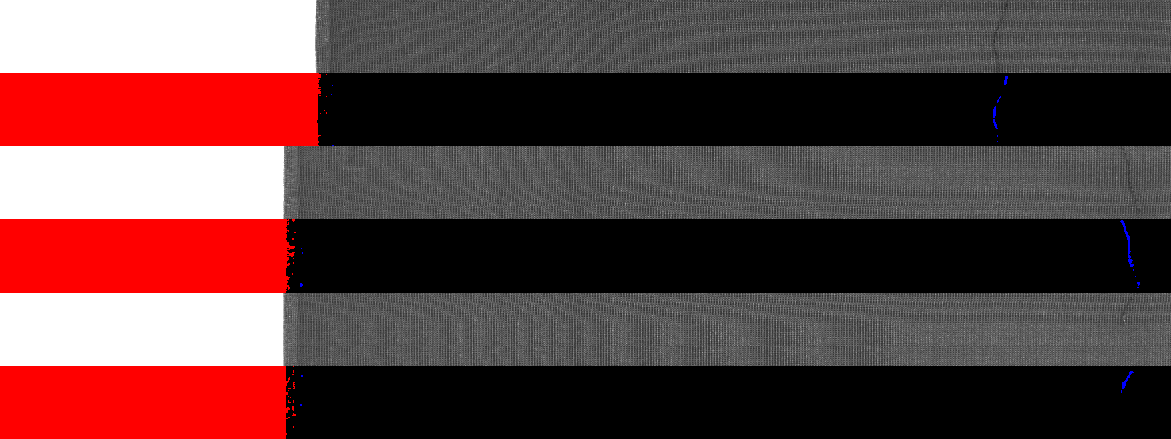
In this article, we’ll use the AITEX Fabric Image Database [1]. It consists of grayscale images of fabric strips with and without defects. The database also includes masks to indicate the location of the defects.


We’ll focus on defects that appear as blobs of pixels with a gray level significantly higher or lower than their surrounding. We will not characterize the fabric texture.
You can find the code used in this article here.
A reasonable approach would be to apply a threshold operation to highlight the bright pixels and an inverse threshold operation to highlight the dark pixels. The threshold value (for both operations) will have to be computed individually since the overall gray level varies a lot from one image to the next.
Uniform thresholding
A good starting point is to evaluate the image median gray level since the median will not be affected much by the left-hand side of the images, where presumably the imaging system scanned columns before the fabric strip reached the camera’s imaging line. The threshold values can then be set by adding (for standard thresholding) or subtracting (for inverse thresholding) a fixed quantity to the gray level median. The magnitude of these delta values will determine how sensitive the threshold operations will be for bright and dark pixels.
We will call this approach _uniform thresholding_ because a single threshold – and inverse threshold – value will be applied uniformly to the image.
We start by blurring the image to attenuate its high-frequency components, assuming that the defects will be larger than a few connected pixels. The Opencv function cv2.blur() implements a uniform averaging of the gray levels in the neighborhood of the central pixel. We choose a neighborhood size that is large enough to make the undesired pattern disappear, but small enough such as sufficiently large defects still stand out clearly from the background.

To compute the median, we call NumPy’s function np.median().
Both the standard threshold and the inverse threshold operations are implemented by the OpenCV function cv2.threshold(). The "type" flag in the function arguments specifies the desired type of operation. We get threshold values for both operations by offsetting the median gray level that we just computed.
After merging the mask of dark pixels with the mask of bright pixels, we get an anomaly mask, highlighting the pixels whose gray level is either dark or bright enough. We obtain good results in some cases if we ignore the left-hand side of the images. It looks like we are only a few tweaks away!
But that is not the end of the story!
As we test more images, we find cases where large areas of the fabric strip are detected as bright or dark, while our judgment tells us that these areas should not be considered abnormal.

We reached the limit of the uniform Thresholding approach. After some investigation, we observe that, in some cases, the average gray level slowly changes as we scan the image from left to right.

The reason could be related to the imaging system. Maybe the images were grabbed with a line scan camera, and the lighting intensity or the integration time was not constant. It could also be related to the product itself: the fabric color could change along the strip. We do not know why, but we must deal with the issue.
A uniform threshold is not enough.
Adaptive thresholding
Adaptive thresholding was invented precisely for this kind of situation. Instead of using a single threshold value for the whole image, each pixel has its threshold value calculated, hence the qualifier adaptive.
For a given central pixel, the gray level weighted average of the pixels in the neighborhood is evaluated. The threshold value is the average gray level, shifted by some constant to provide the desired level of sensitivity. In the output mask, the central pixel gray level is compared to its own personalized threshold.
Adaptive thresholding allows highlighting pixels that are different enough from their neighborhood, instead of simply above or below a uniform threshold.

Back to the fabric image cases for which uniform thresholding did not yield good results, we can find a set of parameters that work much better, with adaptive thresholding (implemented by the OpenCV function cv2.adaptiveThreshold()).

From this point, the next step will be to filter the anomaly mask blobs based on dimension criteria and proximity to other blobs (or machine learning, if we have enough examples). That will present a significant challenge, but at least, with this simple technique, we got rid of artifacts that have nothing to do with defects in the fabric.
Conclusion
In a manufacturing environment where an automated system inspects parts, it is common to encounter cases similar to what we have just observed regarding the non-uniformity of the images. The lighting conditions can vary, the inspected parts can have different colors or reflectivities, multiple cameras can have different sensitivities, the list goes on.
It is essential to design computer vision systems that are robust to these variations, as they are not what the manufacturing engineers and the operators care about: finding the defects without being overloaded by an avalanche of false alarms. Sometimes, something as simple as using adaptive thresholding can help a lot.
[1] AFID: a public fabric image database for defect detection. Javier Silvestre-Blanes, Teresa Albero-Albero, Ignacio Miralles, Rubén Pérez-Llorens, Jorge Moreno, AUTEX Research Journal, №4, 2019


