Thoughts and Theory

The Augmentation Engineers

Augmentations have been around since the early days of deep learning, when we still lacked data. This may be the oldest trick in the book. Why make do with the 20 cat pictures I have in my dataset if, with just a few changes, I can turn every picture into a "new" one? I can move the cat around a bit, zoom and crop, perhaps create a mirror image, rotate it slightly, play around with the color histogram, and lo and behold, I have created a new cat picture! Augmentation has become an integral part of the deep learning training process, so much that only rarely does the model see the original picture. In fact, the model hardly ever sees the same picture twice, because every time a picture needs to be presented to the model, it undergoes such a random combination of transformations, that the chance we might get the same combination using the same picture is practically zero. Here’s to the augmentation combination!

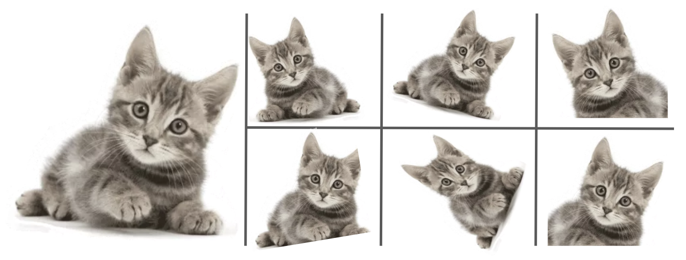
In all these uses, we assume that even if we have altered the image, the change we have made isn’t supposed to affect its essence. The cat is still a cat. Or, if we deal with a medical image of the lungs (a CAT scan?), the tumor is still going to be there if we take a mirror image. By training the model using multiple augmentations of the same picture, yet telling it to predict the same outcome, we really are teaching the model to be impervious to technical changes in the picture which do not alter its essence.

Taking augmentations a step forward, the breakthrough that followed was a surprising one. Why augment only during training? Why not do this on the field, on the product itself? If the algorithm is meant to identify lung tumors, why show it only one picture of the lungs? We can take that same x-ray image, move it around a bit, zoom and crop, perhaps take a mirror image, rotate slightly, play around with the colors, and ask the model to provide a second opinion. And a third. And a fourth. And at the end of the process, we’ll average out all responses. As it turns out, this trick, called Test Time Augmentation, consistently improves a model’s performance by a good few percentage points, so why not?

Enough with the Labels

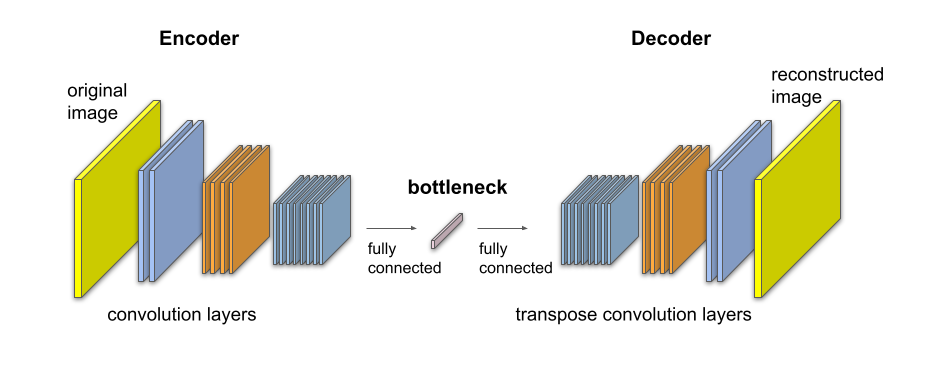
Recent changes in deep learning have placed augmentations front and center. The reason behind this is the holy grail of machine learning – Self-Supervised Learning: learning without any labels. In fact, that’s where we started, when deep learning was at its infancy, and data was scarce. We built autoencoders – models which compress a picture into a small representative vector, a bottleneck, and then expand it back to its full size. We would literally train the model so that the reconstructed image would be as similar to the original as possible, and prayed that all the important image information would be preserved in the bottleneck, without ever guiding the model what is important to preserve. This way we were able to train models on millions of unlabeled images from all around the internet, models which didn’t do much more than to compress an image into a bottleneck vector (commonly referred to as a feature vector) and then extract it back to its original size.

It wasn’t until the second stage that we would turn to our smaller, labeled data set, which contained only a few thousand images, only a few dozen of them were cats, and compress them all into feature vectors using the autoencoder. The belief that this vector also encoded the knowledge of whether the image contained a cat, and that it was encoded there in a way that was easier to extract than in the pixels of the original image, made us think that we would be able to train a non-deep model that wasn’t particularly data-hungry, perhaps just an ordinary SVM, to classify feature vectors into the different classes, and then know whether the image contained a cat or a dog.

But then they built the pyramids. Alongside other new-world wonders, such as Google’s code, Amazon’s warehouses, Apple’s iPhone and Netflix’s streaming, stood the ImageNet project, which holds a data set of millions of images labeled for one thousand object types (including thousands of cat images!). This was the biggest project in 2012 produced by the Mechanical Turk, Amazon’s online trade service. So we bade the autoencoders farewell and began training deep models that directly map an image to its respective class, and results improved greatly.

The compilation of massive, public, labeled data sets has redirected research in this field, since 2012, toward supervised learning. Given that that’s where technological progress took place, many companies have launched mega-operations for collecting and labeling data, sometimes by employing many workers in third-world countries who did little else. For example, it is commonly known that one of Mobileye’s assets is the mechanism for collecting data from the cameras installed in cars, and labeling tens of millions of kilometers of road travel using a designated team based in Sri Lanka. However, most of the data around the world is still unlabeled, and just sits there, waiting for an algorithm to come along that would know how to use it and beat labeled-data algorithms.

Last year, in 2020, it finally happened.

The latest breakthrough in this field stems from an approach called Contrastive Loss, where augmentations play a central role. This is a two-stage approach, working similarly to the way we used the autoencoder’s bottleneck vectors. At stage one we train a model to generate a high-quality feature vector out of every image using a large amount of unlabeled data, and at stage two we train a simple (linear) model using the limited labeled data to classify images.

So how do we teach the model to generate a "high-quality" feature vector? First, what should be the characteristics of such a vector? One of our insights is that we would like to have a vector that is unaffected by augmentation. We said earlier that augmentation doesn’t change the essence of the image, and we want to have a model that is impervious to technical changes in the image which are unrelated to its essence. Unlike the autoencoder, which had to encode at its bottleneck everything that would allow it to recreate an image with identical pixels to those of the original image, and which was therefore sensitive to any possible augmentation, here we would like two augmentations of the same original image to be encoded into the same feature vector.

This resulted in the following training method: we give the model two images, x and x’, after they have been augmented in some fashion. Perhaps x was obtained using a 90-degree rotation of the original image, and x’ was obtained by changing the color histogram. The model is a neural network (like the encoder in the autoencoder) which generates a feature vector out of every image, let’s say y and y’. We don’t tell the model what to put in every such feature vector, but the training loss function imposes an indirect demand – if the two augmentations x and x’ were generated from the same original image we would like the two feature vectors y and y’ to be very similar. Conversely, if the two augmentations were created from two different images, we want their feature vectors to be different from one another.

And so, with every training iteration, we give the computer a batch of different images. We apply two random augmentations to each image, creating image pairs – in some of which the two images originated from the same image, and the model learns to attract their respective feature vectors, and in others, the images were created using different original images, and the model learns to repel their feature vectors. Essentially, the model learns to ignore the augmentation, and to encode into the feature vector only things which are unaffected by it. Things that have to do with the essence of the image, not its technical elements.

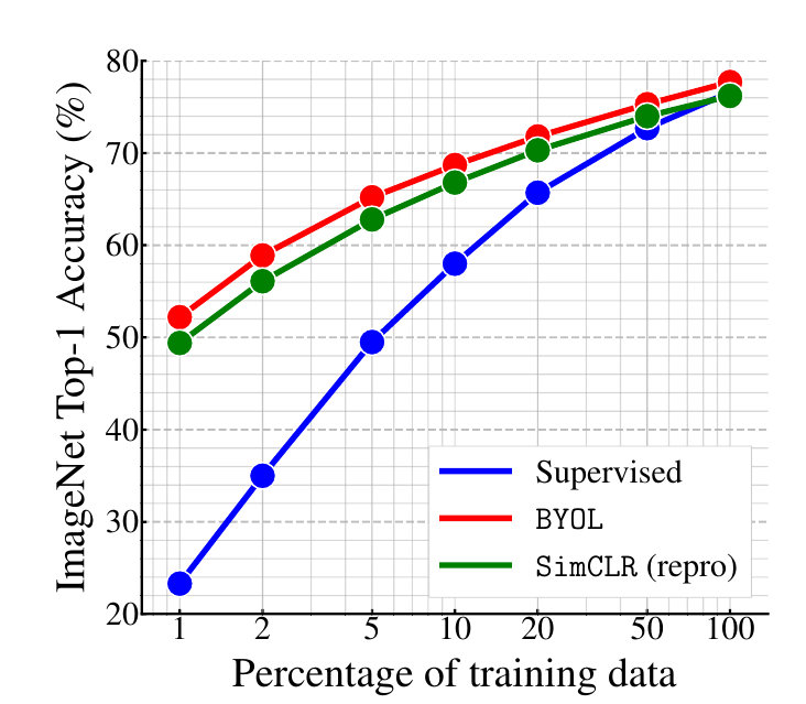
This method gained momentum over the past year, with works such as SimCLR[1] and BYOL[2] (by Google) which bring new tricks to the table, improving the feature-learning process even further, with fewer images residing in every batch. The latest results show that if we treat the ImageNet dataset as a set of unlabeled images and use it for training in stage one, then in stage two we can use only a fraction of the labeled images to reach nearly the same performance as a model which was trained using the fully-labeled ImageNet data. The graphs also show that the contrastive learning approach can get even better if we increase the number of parameters in the model. I am certain that in the coming months we will hear of new ImageNet heights obtained using this method.

Find the Augmentation (and the Anomaly)

Those working in the field of Anomaly Detection have long realized that no ImageNet would ever come to their rescue, and that we would always have to deal with the problem of insufficient data, because the anomaly (for example – a firearm in a luggage x-ray scan) is, by its very definition, a phenomenon which can rarely be found in an organically-curated dataset. In order to deal with this problem, autoencoders were commonly used. If the autoencoder was trained on a large number of suitcases without handguns, and all of a sudden it needs to encode a scan with a handgun into the bottleneck vector, it will have a hard time doing so because the model has never been required to reconstruct an image of a handgun. Therefore, unlike "regular" images, in the case of an image containing a handgun, there will likely be a significant difference between the reconstructed image and the original image, and we can alert security if that is the case. This method worked to a certain extent, and served as the main approach for detecting anomalies for quite some time.

But then another surprising breakthrough came from the realm of augmentation. One thing we can do with a lot of unlabeled data is to label it automatically albeit for a task we aren’t really interested in, such as "find the augmentation". In this game, we pass an image through a single random augmentation out of a collection of (say) 70 possibilities (for example, 180 degrees rotation, 90 degrees rotation, taking a mirror image, zoom and crop, or do nothing); we then present it to the model and ask it to guess which augmentation (out of all the possibilities above) was applied to the image. This is a made up classification task, which although uninteresting by itself, makes use of the unlabeled data, and we can now train a visual model to perform it.

A model that was trained to play this game won’t always manage to detect the correct augmentation. For example, if the image is of an object with a rotational symmetry, such as a flower viewed from the top, then the model will find it hard to detect a 90-degree rotation. If it’s an image of a cat then it would be relatively easy to detect a 90-degree rotation, but a mirror image would still be indistinguishable from a regular image. We can say that the "find the augmentation" model will have a certain confusion signature: some augmentations will be easy to detect, others not so much.

However in their 2018 paper [4], Yitzhak Golan and Prof. Ran El-Yaniv noticed that when a model which has mastered "find the augmentation" gets an anomalous image, the model gets confused in a completely different way than it would in the case of a regular image. In other words, its confusion signature is different. This has resulted in a new method for detecting anomalies: put the suspicious image through all 70 augmentations, and see how many the model can identify. If the confusion signature for the suspected image is sufficiently different from the average confusion signature (estimated from "regular" images), sound the alarm and call security. Surprisingly, this method beats the previously-used autoencoders.

Augmentation Engineers

Deep learning people take pride in the fact that they no longer do feature engineering in order to tell the model how to read the data, and as we transition toward self-supervised learning, we will also be using less and less labels and tags. Nevertheless, we are still engineering something that is crucial to the success of the problem: the augmentations themselves. At the end of the day, if our goal is to distinguish between different types of flowers, then changing the colors of the image as a possible augmentation will prevent the feature vector from containing critical information on the color of the flower. However, if our goal is to distinguish between a "flower" and a "car", then this augmentation works just fine. If our goal is to find a malignant tumor in the lungs which may also appear along their borders, then it would be wrong to crop out parts of the image, because then we might also crop out the tumor, but a mirror image of the lungs would work well. We need to select our augmentation set wisely, in order not to damage the essence of the image for the task we would like to carry out down the line.

In fact, as long as we need to compile the right set of augmentations for contrastive learning, this still is a form of supervised learning, isn’t it? In order to shed this layer, another stage is needed in the training algorithm, which would decide automatically what set of augmentations is appropriate for my data and for the desired task. Until then, having done away with feature engineering, labels, and model architecture, we are still left with the role of "augmentation engineers".

References

[1] Ting Chen, Simon Kornblith, Mohammad Norouzi, Geoffrey Hinton. Simclr: A Simple Framework for Contrastive Learning of Visual Representations. PMLR 2020 [arxiv]

[2] Jean-Bastien Grill, et.al. (DeepMind). Bootstrap your own latent: A new approach to self-supervised Learning. NeurIPS 2020. [arxiv]

[3] Yonglong Tian, Chen Sun, Ben Poole et. al. (MIT, Google). What Makes for Good Views for Contrastive Learning? NeurIPS 2020 [pdf]

[4] Izhak Golan, Ran El-Yaniv. Deep Anomaly Detection Using Geometric Transformations. NIPS 2018. [arxiv]