Mastering Dynamic Programming

Are you anticipating a job interview with big tech companies like FAANG? If so, be prepared to go through one or more rounds of technical coding assessments.

In fact, a growing number of firms have started to include technical coding assessments in their interview process for the data scientist, machine learning engineer, or software engineer roles.

Such assessments usually test candidates on database and data manipulation skills with SQL, or problem-solving and programming skills with data structures and algorithms. The latter often include dynamic programming, an optimization technique that can produce efficient codes with reduced time or space complexity.

Let’s get moving and gear up on dynamic programming.

---

Contents

1. Characteristics of Dynamic Programming 2. Types of Dynamic Programming Questions 3. Approaches to Implement Dynamic Programming ∘ Top-Down Approach ∘ Bottom-Up Approach 4. Dynamic Programming Examples ∘ Example 1: Climbing Stairs ∘ Example 2: House Robber ∘ Example 3: Cherry Pickup What’s Next? Summary

1. Characteristics of Dynamic Programming

Many of us face the difficulty of identifying a dynamic programming problem. How do we know if we can solve a problem with dynamic programming? Well, we can ask ourselves the following questions.

• Can we break down the problem into smaller sub-problems?
• Are there any overlapping sub-problems?
• If yes, can we solve the smaller sub-problems optimally, and then use them to construct an optimal solution to solve the main problem?
• While solving the problem, does the decision on the current step affect the outcome and decision of subsequent steps?

If your answer is Yes to the above questions, then you can apply dynamic programming to solve the given problem. According to Wikipedia,

"There are two key attributes that a problem must have in order for dynamic programming to be applicable: optimal substructure and overlapping sub-problems"

Do not confuse Dynamic Programming with Divide-and-Conquer or Greedy algorithm.

Divide-and-Conquer also solves a problem by combining optimal solutions from sub-problems. However, the sub-problems in Divide-and-Conquer are non-overlapping.

A Greedy algorithm would try to make a greedy choice to provide locally optimal solution for each step. This may not guarantee that the final solution is optimal. Greedy algorithm would never look back and reconsider its choices, while dynamic programming may revise its decision based on reviews of previous steps.

2. Types of Dynamic Programming Questions

What do dynamic programming questions look like?

Let’s check out some of the most common types of dynamic programming questions.

The first type of dynamic programming question, which is also the frequently encountered kind, is to find an optimal solution for a given problem. Examples include finding the maximum profit, the minimum cost, the shortest path, or the longest common subsequence.

The second type of dynamic programming question is to find the possibility of achieving a certain outcome, the possibility of reaching a certain point, or the possibility of completing a task within the specified conditions.

The third type is usually referred to as a dynamic programming counting problem (or combinatorial problem), such as finding the number of ways to perform or accomplish a task.

Note that all three types of dynamic programming questions that we discussed could also appear as two-dimensional problems in the form of a matrix. More complex problems could involve multiple dimensions.

3. Approaches to Implement Dynamic Programming

We can solve dynamic programming problems with the bottom-up or top-down approach. Regardless of which, we need to define and come out with the base case of the problem.

Generally, the top-down approach starts by looking at the big picture. From the high level, it gradually drills down into the solution for smaller sub-problems, and finally, the base case for constructing the solution.

As opposed to the top-down approach, the bottom-up approach starts small by first looking at the base case, and from there step-by-step building up the solution to bigger sub-problems, before solving the entire problem as a whole.

Imagine the following:

Top-down: "I want to make a delicious, gorgeous-looking birthday cake. How to achieve that? Hmm…I can make use of luscious Chantilly cream, berries compote, flowers, and fresh strawberries to decorate the cake. How to prepare them? I need to whip the heavy cream with sugar, cut the strawberries and cook the berries compote. But where’s the cake? Oops, I need to prepare the cake batter and bake it. How? Whip the butter with sugar and egg, then mix in the flour and milk. How much to use for each ingredient? I need to measure them based on the required proportions".

Bottom-up: "I will start by measuring and preparing the cake ingredients. With all the ingredients ready, I whip the butter with sugar and egg before mixing in the flour and milk. Next, I put it into the oven and bake for 30 minutes. After baking the cake and letting it cool down, I cook the berries compote, cut the fresh strawberries, and whip the heavy cream with sugar. Thereafter, I frost the cake with the Chantilly cream, spread the berries compote on top, and finally put on and arrange the cut strawberries and edible flowers".

Can you notice how the bottom-up approach does things in an orderly fashion starting from the basics?

Top-Down Approach

The implementation of a top-down approach uses recursion with memoization.

Memoization is the technique of storing the result of calculations so that they can be retrieved and used directly when the program requires them again. This is especially useful for overlapping sub-problems as it helps to avoid performing the same calculation twice, thus improving efficiency and saving compute time. Hashmap or array are commonly used for memoization.

This approach will make recursive function calls as per the recurrence relation that we define, as long as the current state is not the base case.

Bottom-Up Approach

To implement the bottom-up approach, we would need to iterate over all the states of the problem in a specific order, starting from the base case.

By doing so, we build up the solution step by step from small to big, such that the answer for the current step can easily be computed using the available sub-problem solutions computed from the earlier steps. This process keeps going until we build up the entire solution.

The bottom-up approach is also known as the tabulation method. Since this approach would go through each step in a specific order and perform computation, it is easy to tabulate the results in an array or list, where they can be conveniently retrieved by the relevant index for use in subsequent steps.

For some scenarios, tabulation can be avoided to save space and memory. We would see this in Example 1 and Example 2 later.

So which approach to use?

It’s generally fine to use either approach. After all, dynamic programming is not easy to comprehend. You can use whichever approach that comes more naturally to you, and the one you’re more comfortable with.

While some may find it easier to frame a solution with recurrence relation and code using the top-down approach, the bottom-up iterative process could sometimes execute faster as it does not have the stack overheads of recursion. Most of the time, the difference is just marginal. If you’re skillful and able to code both, needless to say, go for the one that has less time and space complexity.

4. Dynamic Programming Examples

In this post, we will go through in great detail three examples of solving dynamic programming problems.

Example 1: Climbing Stairs

Let’s start with an easy-to-understand example, Climbing Stairs.

In this problem, we are given a staircase that would take us n steps to reach the top. Each time, we are only allowed to climb 1 step or 2 steps.

In how many different ways can we climb to the top?

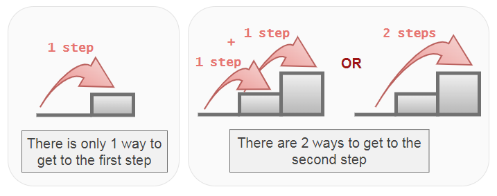
Let us begin by thinking about the base case. If we were to get to the first step, how many ways can we do that? Of course, there is only 1 way, and that is to climb 1 step.

How about getting to the second step? There are 2 ways to accomplish this. We can either climb 1 step twice, or we can climb 2 steps once.

Good! Getting to the first step and getting to the second step constitutes the base case for this problem. Now, how about the third step, the fourth step, and so on?

For the third step, there are just 3 possible ways to reach there. They are:

• climb 1 step for 3 times, or
• climb 1 step followed by 2 steps, or
• climb 2 steps followed by 1 step

And how do we get this number? It’s by adding the results from the first step and the second step (1 + 2 = 3). This tells us that from the base case, we can construct solutions to the other steps. Assuming climb(n) is the function that returns the number of ways to reach step n, then

climb(n) = climb(n-1) + climb(n-2)

And there we have it, it’s the recurrence relation for this Climbing Stairs problem. The current step takes the computations from the previous two steps and sums them.

Basically, this is how we break down a problem into sub-problems, and solving the sub-problems will construct a solution to the main problem.

Can you see that these sub-problems are overlapping?

climb(6) = climb(5) + climb(4)
climb(5) = climb(4) + climb(3)
climb(4) = climb(3) + climb(2)
climb(3) = climb(2) + climb(1)

To get the result of climb(6), we need to compute climb(5) and climb(4). And to get the result of climb(5), again we need to compute climb(4).

We can clearly see from the figure below that in order to get climb(6), we have to compute climb(4) two times, and compute climb(3) three times. This will result in having a time complexity of O(2^n).

With memoization, we can get away with redundant computations and just retrieve the previously-stored results. Time complexity will be reduced to O(n).

Alright, we have the base case and the recurrence relation, now it’s time to write the implementation using the top-down approach.

Here, for memoization, we use a hashmap (Python dictionary) to store the results of computations. If result for n exists, we skip the computation and retrieve the result from the hashmap.

Both the time and space complexity for this approach is O(n). This is because we are literally going through every step, and for each step, we’re storing the computation result in the hashmap.

Below is the solution using the bottom-up approach.

Typically, we can use an array to tabulate the computed values for each step. However, for this problem, since the current state depends only on the previous two states, we can efficiently just use two variables, case1 and case2, to keep track of them while iterating the for loop.

By doing so, we are able to achieve a constant space complexity, O(1). Time complexity will be the same as the top-down approach, O(n).

Example 2: House Robber

This is another classic example of a dynamic programming problem, House Robber.

In this problem, we’re given an array of integers, representing the amount of money in each house that a robber can rob. The houses are lined up on a street. There is one constraint though, that the robber cannot rob adjacent houses. For example, if the houses are indexed from 0 to 4, the robber can rob houses 0,2,4, or houses 1,3.

What is the maximum amount of money that the robber can rob from the houses?

Let’s walk through with a sample input of house = [10, 60, 80, 20, 8].

Again, we start by thinking about the base case. If there is only one house, house[0], what would we do? We would just rob and take the money from house[0]. This is because there is no other choice to consider.

Now, if we have two houses, house[0] and house[1], which one do we rob? We cannot rob both houses since they are adjacent to each other. We can either rob house[0] or house[1]. Well, of course, we will rob the house containing more money. To find the house containing more money, we apply max(house[0], house[1]).

Notice how the above forms the base case for this problem?

Now, what if there are many houses? What do we do then? Let’s think of it this way. If we’re at house[n], we have two options, i.e. whether to rob, or not to rob the house.

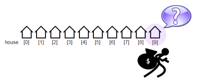
• Let’s say we’re at house[9]. If we decide to rob house[9], then what we would get is the amount of money from house[9] plus whatever the amount that we got up to 2 houses before.
• If we decide not to rob house[9], then what we have is simply the amount we got from robbing the houses up to house[8].

To find out which option yields the maximum amount of money, we apply the max() function on these two options, and that makes our recurrence relation:

rob_house(n) = max(rob_house(n-2) + house[n], rob_house(n-1))

With the base case and recurrence relation on hand, we can now write the solution using the top-down approach. The time and space complexity for this approach will be O(n).

For the bottom-up approach, instead of tabulating an array, again, we use two variables, case1 and case2 to keep track of the previous two states.

Remember the base case when there is only one house, and when there are two houses? case1 is initialized with the value from the first house, and case2 is initialized with the result of max(house[0], house[1]).

The figure below illustrates the workouts when we have 3 houses.

For the third house where n = 2, and for subsequent iterations, we can compute the result by applying max(case1 + house[n], case2). Because we’re recycling the two variables, case1 would be replaced by case2 after the current computation, and the result of the current computation would be assigned to case2.

Using only two variables allows us to achieve a constant space complexity, O(1). Time complexity will be the same as the top-down approach, O(n).

Example 3: Cherry Pickup

Let’s attempt a more challenging problem, Cherry Pickup.

In this problem, there is a n x n grid where the value in each cell can either be 1 (there’s a cherry in the cell), 0(the cell is empty), or -1(there’s a thorn, an obstacle that blocks the way).

Starting at cell (0,0), we are supposed to move to the destination, which is located at (n-1, n-1). If there are cherries along the way, we pick them up. If we pick up cherry from a cell, the cell becomes an empty cell, 0. We are only allowed to move down or right, and if there’s a thorn, we will not be able to pass through.

After reaching the destination at (n-1, n-1), we have to do a return trip to the starting cell (0,0). For the return trip, we are only allowed to move up or left, picking up remaining cherries, if any.

If we can’t find a way to reach the destination at (n-1, n-1), then we can’t collect any cherries.

We are asked to return the maximum number of cherries we can collect.

On first thought, what comes to our mind is to model a solution to pick up the cherries on a forward trip followed by a return trip, as articulated by the problem.

But, let’s try a novel approach with the methodologies adopted from here.

That is, instead of a forward trip followed by a return trip, we will traverse only on a forward trip. Why? It’s because the forward trip practically works the same as the return trip in this problem. In other words, we can traverse the same path on a forward trip that can only move down or right️, as well as on the return trip that can only move up or left️. Does that make sense?

Next, instead of making two trips, we can simply just do a single forward trip with the idea of two persons moving simultaneously. Thus, at any point in time, the two persons would have made the same number of moves.

Assuming person1 is at position (r1,c1) and person2 is at position (r2,c2) after a certain number of moves, we have r1 + c1 equal to r2 + c2. Sounds bizarre? Take a look at the illustration below.

This means we can use r1, c1, r2, c2 as state variables in our problem. But do we really need all four of them? With a grid of length n, it would result in O(n⁴) states.

We can improve and reduce the state variables to just three, i.e. r1, c1, c2. But how about r2? Well, we still need r2, and we can derive its value from the equation. This state space reduction will bring down the time and space complexity of this problem from O(n⁴) to O(n³).

r1 + c1 = r2 + c2

Derive r2 as:
  r2 = r1 + c1 - c2

Where
  r1 is the row index of person1
  c1 is the column index of person1
  r2 is the row index of person2
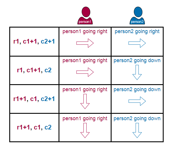
  c2 is the column index of person2

So, how do the three state variables work out in this problem? Since we have two persons moving simultaneously, there are four possibilities for each move, as depicted below:

Now, after having a clear understanding of the concepts and with enough information, let’s build the top-down solution.

This time, instead of using hashmap for memoization, we are going to use Python’s [lru_cache()](https://docs.python.org/3/library/[functools](https://docs.python.org/3/library/functools.html#module-functools).html#functools.lru_cache) decorator from the functools module.

In our solution, we will create a get_cherry() recurrence function and use a variable called cherries to accumulate the cherries picked.

Presuming person1 is at position (r1,c1) and person2 is at position (r2,c2), and there are no thorns at both locations, we first add the value from (r1,c1) to cherries. Because there is no thorn, the value is either 0 or 1.

Next, to avoid double-counting, we would add the value from (r2,c2) to cherries only if person2 is at a different location.

So far, what we’ve done is accumulate cherries on the current location of person1 and person2. We would need to do the same accumulation for subsequent locations too.

Remember earlier we said that there are four possibilities for each move? To determine which path to take in order to get the maximum number of cherries for subsequent locations, we can apply the max() function on the four options. This forms the recurrence relation for this problem.

The recursive function calls would continue until the destination cell is reached. When that happens, the function would return the value of that cell. As this is the base case, no further recursive function calls would be made.

Wow! That’s a perfect plan, isn’t it? But there are exceptions.

What if there is a thorn at (r1,c1) or (r2,c2)? And what if person1 or person2 goes out of bound?

Obviously, we want to avoid those places as much as possible. If that happens, the function would return a negative infinity, signifying that the particular path is not worth taking for finding the optimal answer. Negative infinity is essentially the minimum, so the max() function would take on another option that has the largest value.

And lastly, what if person1 or person2 is not able to reach the destination? Well, this is possible and it could happen due to thorns obstruction. In this case, no cherry can be collected, and the final answer would be 0.

For this problem, I’ll leave it to the intrigued reader to think about the bottom-up solution. Who knows, you might be able to come out with a fantastic solution.

What’s Next?

By all means, go and practice solving dynamic programming problems.

Take the first step. If you’re not able to crack the solution, fret not. Check out some of the discussion forums, where you can usually find useful tips and guidance.

The most well-known platform where you can practice is LeetCode. Others include GeeksforGeeks, HackerEarth, and HackerRank.

The more we practice, the more we learn. The more we learn, the easier it gets!

Summary

☑️ In this post, we went through the characteristics of dynamic programming and the key attributes for dynamic programming to be applicable.

☑️ We unveiled the typical types of dynamic programming questions that are often being asked.

☑️ We explored the differences between the top-down and bottom-up approaches, and in what manner to implement them.

☑️ We learned how to solve dynamic programming problems by running through 3 examples that include detailed explanations and solutions.

References

[1] LeetCode, Climbing Stairs, House Robber, Cherry Pickup

[2] GeeksforGeeks, Dynamic Programming

[3] Prateek Garg, Introduction to Dynamic Programming 1

[4] Programiz, Dynamic Programming

---

Dynamic programming is fun. Some of the problems could be intimidating and mind-boggling, but learning to solve them and mastering the skills can open up a rainbow of possibilities!

---

Before You Go...

Thank you for reading this post, and I hope you've enjoyed learning dynamic programming as much as I do. Please leave a comment if you'd like to see more articles of this nature in the future.

If you like my post, don't forget to hit Follow and Subscribe to get notified via email when I publish.

Optionally, you may also sign up for a Medium membership to get full access to every story on Medium.

📑  Visit this GitHub repo for all codes and notebooks that I've shared in my post.

© 2022 All rights reserved.

Ready to dive deeper? Hop on to Mastering Dynamic Programming II

Mastering Dynamic Programming II

Interested to read my other Data Science articles? Check out the following:

Transformers, can you rate the complexity of reading passages?

Advanced Techniques for Fine-tuning Transformers

AWS Certified Machine Learning – Specialty

Building a Product Recommendation Engine with AWS SageMaker