Machine Learning: Target Feature Label Imbalance Problem and Solutions

Getting Started

Table of Contents

Part 1: Concepts

1. Introduction
2. What is train data?
3. Why do we need to balance train data?
4. What does "balancing data" actually look like in practice?
5. Do we also need to balance test data?
6. Evaluation metrics for imbalanced test data

Part 2: Code

1. Setup
2. Initial feature engineering
3. Model purpose transformation
4. Addressing categorical features
5. Train test split
6. Data balancing
7. Models
8. What if we balance the test data?
9. Conclusion
10. Resources

---

Part 1: Concepts

1. Introduction

The goal of this post is to teach python programmers why they must have balanced data for model training and how to balance those data sets. Often times, in machine learning classification problems, models will not work as well and be incomplete without performing data balancing on train data. This post will serve as an end-to-end guide for solving this problem.

Table of contents

---

2. What is train data?

Before running a model, you need to fit the model on a set of data that is distinct from the data you test it on. In other words, if you create a model based on one pool of data and run that same pool of data back through the model, and the model performs well, you likely haven’t built anything exciting or proven anything. Therefore, a common way to generate extra data is to cut off a random segment of the total data, and use the remaining data for model training and go back to the cut off (and smaller) set of data for model validation purposes.

Table of contents

---

3. Why do we need to balance train data?

I am a strong believer in using extreme examples to prove points. In this case, I’d like to provide the following example to demonstrate why data balance matters in classification algorithms: say you are trying to predict whether a certain disease is likely to occur for a given person. Let’s focus on the output here, meaning the y-value we are trying to predict via our numerous features. Make up all the features you want to use as they won’t matter in a second. If we had 500 data points and 499 showed healthy people while 1 showed a diseased person and our model had 100% accuracy… well it doesn’t prove a whole lot. In fact, it proves just as much as a 99.99% accurate model where the one error was in the diseased person predicted as healthy. Having a 499-to-1 distribution of data points just doesn’t cut it as we don’t have the required level of data to develop an understanding of what may lead to disease. Balancing data gives us the same amount of information to help predict each class and therefore gives a better idea of how to respond to test data.

Table of contents

---

4. What does "balancing data" actually look like in practice?

There are a couple ways to think through balancing data. I will talk about three in particular. I’ll start by discussing the ideas here and later share the coding process.

Example data:

10 rows of data with label A.

12 rows of data with label B.

14 rows of data with label C.

Method 1: Under-sampling; Delete some data from rows of data from the majority classes. In this case, delete 2 rows resulting in label B and 4 rows resulting in label C.

Limitation: This is hard to use when you don’t have a substantial (and relatively equal) amount of data from each target class.

Method 2: Copy rows of data resulting minority labels. In this case, copy 4 rows with label A and 2 rows with label B to add a total of 6 new rows to the data set.

Limitation: I think the limitation here is pretty clear. All you are really doing is copying current data and you don’t really present anything new. You will get better models, though.

Method 3: (SMOTE – Synthetic Minority Oversampling Technique) Synthetically generate new data based on implications of old data. Basically, instead of deleting or copying data, you use the current inputs to generate new input rows that are unique but will have a label based on what the original data implies. In the case above, one simple way to think of this idea would be to add 4 rows with label A to the data where the inputs represent total or partial similarities in values to current input features. Repeat this process for 2 rows of label B as well.

Limitation: If two different class labels have common neighboring examples, it may be hard to generate accurate data representing what each unique label may look like from the input side and therefore SMOTE struggles with higher dimensionality data (Lusa, L and Blagus, R, 2013).

Table of contents

---

5. Do we also need to balance test data?

Usually, this is something we don’t do. You can sometimes upsample test data anyway just to see if your model works well on minority classes as well. What’s most important to keep in mind is that you don’t want to upsample data and only then do a data split into train and test set. This will likely result in having elements of train data copied perfectly into test data and artificially boost your model scores. The only time you would ever upsample test data is after a data split, just like you only perform data balancing on train data.

Table of contents

6. Evaluation metrics for imbalanced test data

If we have a strong imbalance in test data, we still have ways of understanding how well our model performs outside of the accuracy metric. Accuracy, our intuitive and classic metric, is actually only a measure of wrong-or-right for every single observation. It does not take into account how many of each label are included in the data and works best with relatively balanced data (or in cases where correct predictions are more important regardless of the distribution of the various outcomes in the target feature). Having alternative metrics is less of a reason as to why you shouldn’t balance test data, but more of a reason why you might not need to balance test data. Let’s look at three metrics that are effective in the context of binary classification algorithm (they are also relevant for non-binary problems, but binary problems provide the easiest method of illustration).

Precision

Precision is a measure that tells you how meaningful a positive (target class = 1) is. This is accomplished by dividing the number of correct positive predictions over total number of positive predictions (true positive divided by sum of false positives and true positives). Say you are predicting disease and have 400 healthy people and 100 diseased people. If you predict all 500 cases to be diseased, you have correctly identified every case of disease, but your model is rather meaningless as you always have the same outcome and you misidentified 80% of the inputs.

Recall

Recall is very similar to precision. The denominator in recall, however, is composed of true positives and false negatives, while the numerator remains true positives. This shifts our focus from how much a positive score actually matters, to an understanding of how effective our model is at identifying any positive case that is present (because a false negative is actually a positive). As the number of false negatives grow, there is no increase to the numerator of true positives, and the recall gets lower and lower. Let’s use the precision example again. If you predict 500 patients to be diseased when only 100 are actually diseased, you will have high recall as there are no false negatives. However, if you go to the other extreme and say everyone is healthy, then all the sudden you have 80% accuracy and no false positives but you failed to identify 100% of the diseased people. You may notice that in the case where everyone is predicted to be sick that precision is low while recall is high. There is in fact a moderate tradeoff between optimizing precision and recall.

F1-Score

The F1-Score is the perfect way in which we can get a better sense of model performance when we have imbalanced data since accuracy alone isn’t a good metric. F1-Score is a harmonic average (max value is the arithmetic mean) of the precision and recall score. Having a blend of precision and recall gives us a strong idea of how well the model actually works.

Table of contents

---

Part 2: Code

The data I will be using for demonstration can be found at kaggle.com at this link and deals with diamond price prediction

The code below will take you through the entire process; from beginning imports and data preparation to modeling

1. Setup

• Install libraries

!pip install -U scikit-learn
!pip install -U imbalanced-learn
!pip install xgboost

• Import necessary libraries

# remove warnings
import warnings
warnings.filterwarnings('ignore')

# standard imports and setup
import pandas as pd
import numpy as np
import matplotlib.pyplot as plt
%matplotlib inline
import seaborn as sns
from scipy import stats

# model evaluation
from sklearn.model_selection import train_test_split, cross_val_score, GridSearchCV, ShuffleSplit
from sklearn.metrics import *

# pipelines
from sklearn.compose import make_column_transformer
from sklearn.pipeline import Pipeline, make_pipeline

# data preparation
from sklearn.preprocessing import *
from sklearn.decomposition import PCA
from sklearn.feature_selection import RFE, RFECV
from sklearn.utils import resample
from imblearn.datasets import make_imbalance
from imblearn.over_sampling import SMOTE

# machine learning
from sklearn.linear_model import *
from sklearn.neighbors import KNeighborsClassifier
from sklearn.svm import SVC, LinearSVC
from sklearn.naive_bayes import GaussianNB
from sklearn.ensemble import RandomForestClassifier, RandomForestRegressor
from sklearn.tree import DecisionTreeClassifier
from xgboost import XGBClassifier, XGBRegressor

• Read and preview data

df=pd.read_csv('diamonds.csv')
print(df.shape)
df.head()

• Drop "Unnamed: 0" as it is useless and look for null values
• While looking for null values, get a feel for the data types

df.drop('Unnamed: 0', axis=1, inplace=True)
df.info()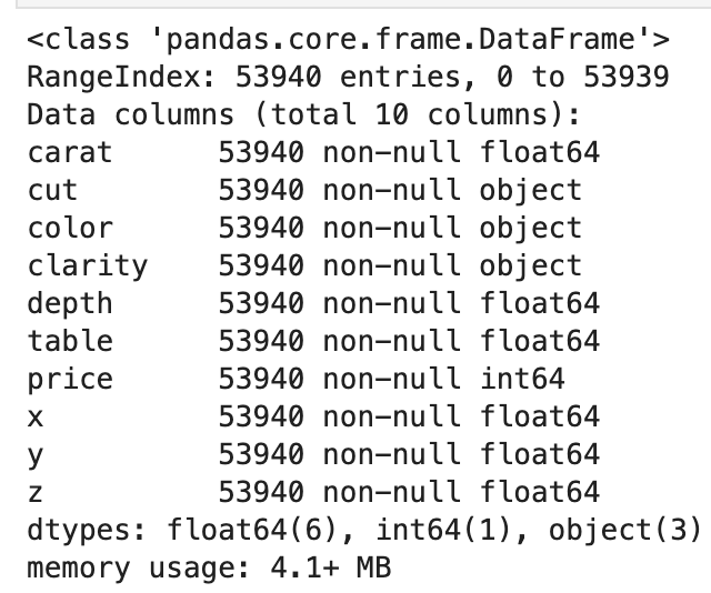

• There appear to be no null values

Table of contents

---

2. Initial Feature Engineering

• Next, we will quickly do some feature modifications
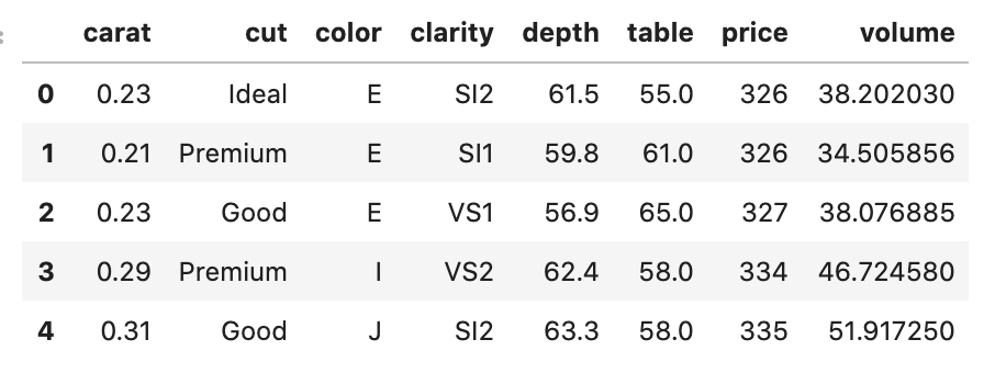
• You may notice that the product of x, y, and z (according to the kaggle link) correspond to volume. We can add a feature called volume to equal this product and remove x, y, and z. I’d like to credit Chinmay Rane for this idea as I saw it in his kaggle notebook which can be found at this link (Rane, 2018)

df['volume'] = df.x*df.y*df.z
df.drop(['x','z','y'],axis=1,inplace=True)

• What does new data look like?

Table of contents

---

3. Model Purpose Transformation

• You may notice that the data above present our target feature of price as a continuous variable, but we can establish sets of intervals in the target feature to morph it into a classification problem
• The plan is as follows: we will split the target feature into various intervals of values, and I like picking four unique intervals for this problem
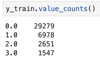
• Those intervals are as follows (along with value counts)

• Pandas has a built in function to break things down into bins and you can even have a 1:1 ratio from each bin size to the next using pd.qcut
• We still have a problem as it is a bit of a pain to look at intervals
• Thankfully, Pandas let’s users create default labels as I will show below

df['price_bin']=pd.cut(df.price,bins=4,labels=[0,1,2,3])

• Now, look at data below from the first couple rows
• You may notice that the most common label above is 0 and that is reflected below

• For more information on the built-in functions used above, you can view documentation for pandas.cut [here](https://pandas.pydata.org/pandas-docs/stable/reference/api/pandas.qcut.html#pandas.qcut) and documentation for pandas.qcut here

Table of contents

---

4. Addressing Categorical Data

• We now are looking at a classification problem, but there is still the problem of the features cut, color, and clarity which do not have numeric values
• To solve this problem we will use label encoding which is a method of assigning a numeric label for unique value of a categorical variable
• I actually prefer target encoding, but don’t believe target encoding is the most "fair" approximation with very few input features present
• After encoding labels, we will do a double check to ensure our data is of type float

le = LabelEncoder()
for col in df.select_dtypes(include='O').columns:
    df[col]=le.fit_transform(df[col])

for col in df.columns:
    df[col]=df[col].astype(float)

For more information on label encoding using python, you can view the documentation

Table of contents

---

5. Train Test Split

• Now that our data is prepared, we will have to split the data into two sets for reasons described above
• To accomplish this, we will first assign the X values to everything but the output feature (aka all the inputs)
• Next, we assign y values to the price_bin feature; our modification of the price feature
• Finally, we assign X_train and y_train together as a "matching dataset" and do the same for X_test and y_test
• We will then fit a model using X_train and its outputs y_train and validate the model by comparing predictions based on X_test to actual output of y_test

X = df.drop(['price','price_bin'],axis=1)
y = df.price_bin
X_train, X_test, y_train, y_test = train_test_split(X,y)

For more information on train_testsplit, you can view the documentation_

Table of contents

---

6. Data Balancing

• Ok, take a breath; we’ve finally made it to the data balancing

Method 1

• We see below the distribution of the target class in our data in both train and initial sets

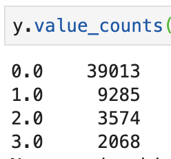
• What we see here is that the lowest we can go for each class to be equal is around 2000
• I’m going to go with 1500 though
• Using make_imbalance from imblearn, we can easily just delete rows to balance the classes (more information on this process can be found at the _documentation_)

• I will store these new values into X_train_1 and y_train_1 so we can see which method works best at the end when we run all the models

• Having balanced our data, let’s see the outcome by running the following code

y_train_1.value_counts().plot(kind='bar')
plt.title('label balance')
plt.xlabel('label values')
plt.ylabel('amount per label')
plt.show()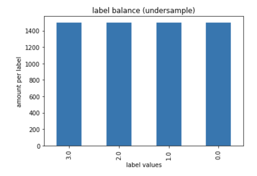

Method 2

• For method two, we will copy existing rows of minority classes using resample from sklearn.utils
• I wrote the function below to help you easily accomplish this task (but the key part of the function is the resample import and information on this function can be found at the documentation)
• There is, however, a prerequisite that you need to combine X_train with y_train and only then upsample classes

Creating upsample_classes function

• Input is data and what the target feature from that data is
• Output is a balanced dataset
• First, we make a list of unique labels in data
• Next, we split up the rows of data by their labels into different sets of data
• Next, we search for the majority class label
• Next, we get the classes back together using pandas.concat (more on this function can be found at the documentation) and separate off the majority class based on it’s newly found label
• Next, we remove the majority class and upsample the other classes to match the length of the majority class

• Finally, we combine the majority class with the other classes, which are now of equal length

• This function is very simple due to the fact that there are only two inputs
• Let’s see how to turn this into new sets of X_train and y_train

train = pd.concat([X_train,y_train],axis=1)

train_balanced = (upsample_classes(train,'price_bin'))

X_train_2 = train_balanced.drop(['price_bin'],axis=1)
y_train_2 = train_balanced.price_bin

• Outcome

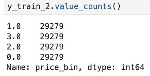
• Visual

y_train_2.value_counts().plot(kind='bar')
plt.title('label balance')
plt.xlabel('label values')
plt.ylabel('amount per label')
plt.show()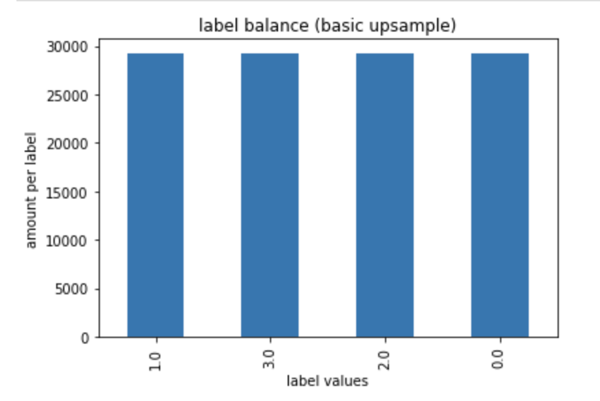

Method 3 (SMOTE)

• While the actual calculations and backend for SMOTE are beyond the scope of this post (but is discussed elsewhere on the internet), we will use python and its libraries to leverage the SMOTE technique with only a couple lines of code (Doken, S)
• Recall that SMOTE can be thought of a way of synthetically generating new data based on what other rows of data may imply
• All you need for SMOTE is two lines of code and you can learn more about the specifics of SMOTE in python at the _documentation_

smote = SMOTE(random_state = 14)
X_train_3, y_train_3 = smote.fit_sample(X_train, y_train)

• Now you have balance in the target class, as we will see below

y_train_3.value_counts().plot(kind='bar')
plt.title('label balance')
plt.xlabel('label values')
plt.ylabel('amount per label')
plt.show()

• That wasn’t too bad!

Table of contents

---

7. Models

• We need to start this section with a disclaimer: the dataset here is a fairly simple dataset and contains few features. Just because some models paired with different data balancing methods may work here in certain ways here, they may look different in different datasets and different scenarios
• We start by instantiating our modeling technique (my lucky number is 14)
• We will also only use XGBoost for uniformity purposes (and it works very well, anyway)
• To learn more about XGBoost classifiers in python, you can view the _documentation_

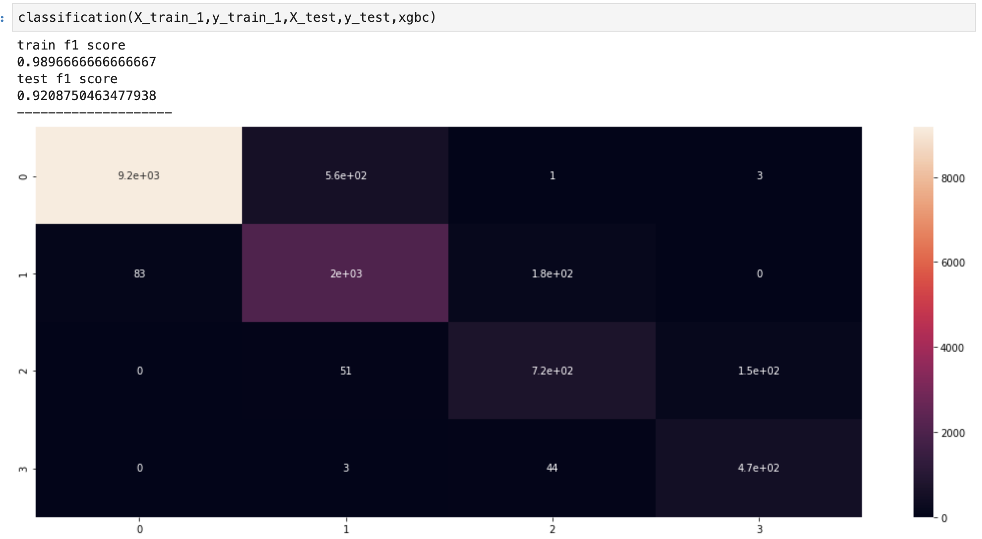
xgbc=XGBClassifier(random_state=14)

• To make life easy and to avoid writing everything over and over again, I will also create the following function

Creating classification function

• Input train data, test data, and a model type
• Start by fitting model on train data
• Assign prediction variables for train and test set
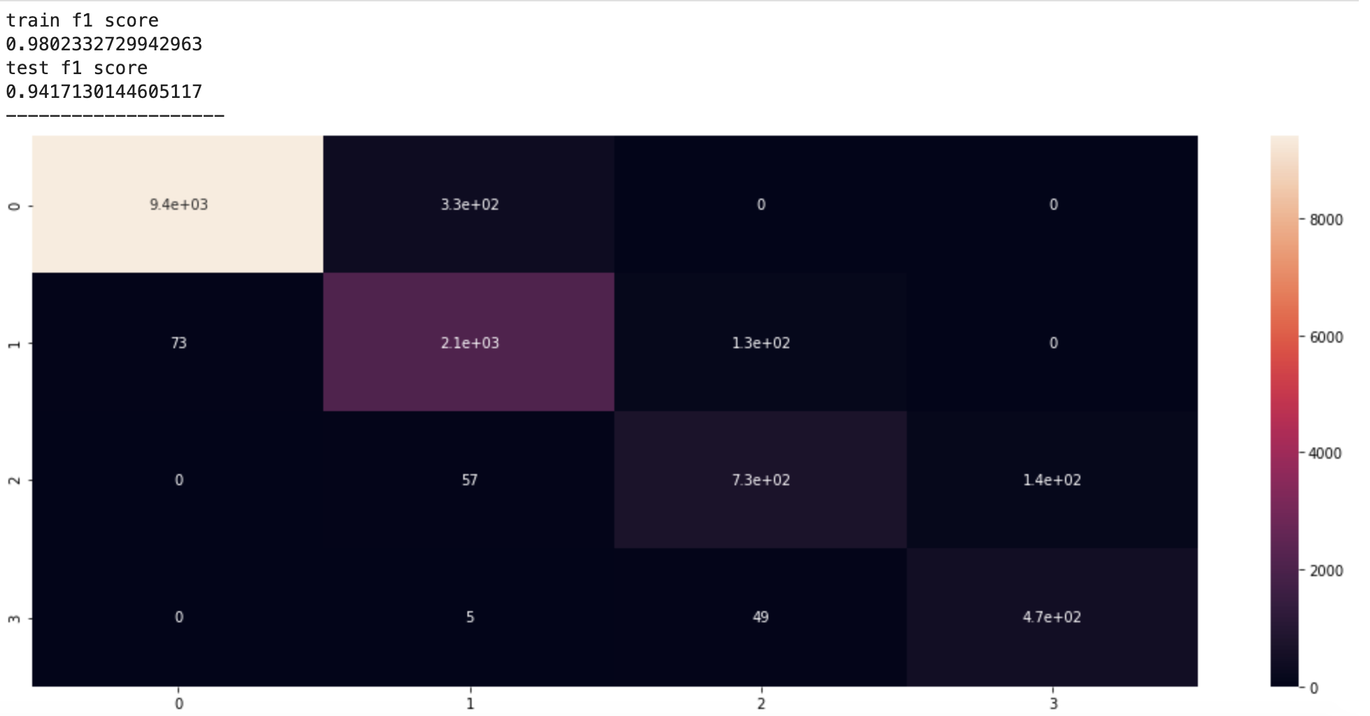
• Due to class imbalance in test data, display f1 score for train and test predictions using scikit-learn’s built in metrics library (more information on F1 score can be found at the _documentation_)

• Display a confusion matrix for performance of test data (more information on confusion matrices in python can be found at the _documentation_)

• Let’s run through the results

Method 1

Method 2

Method 3

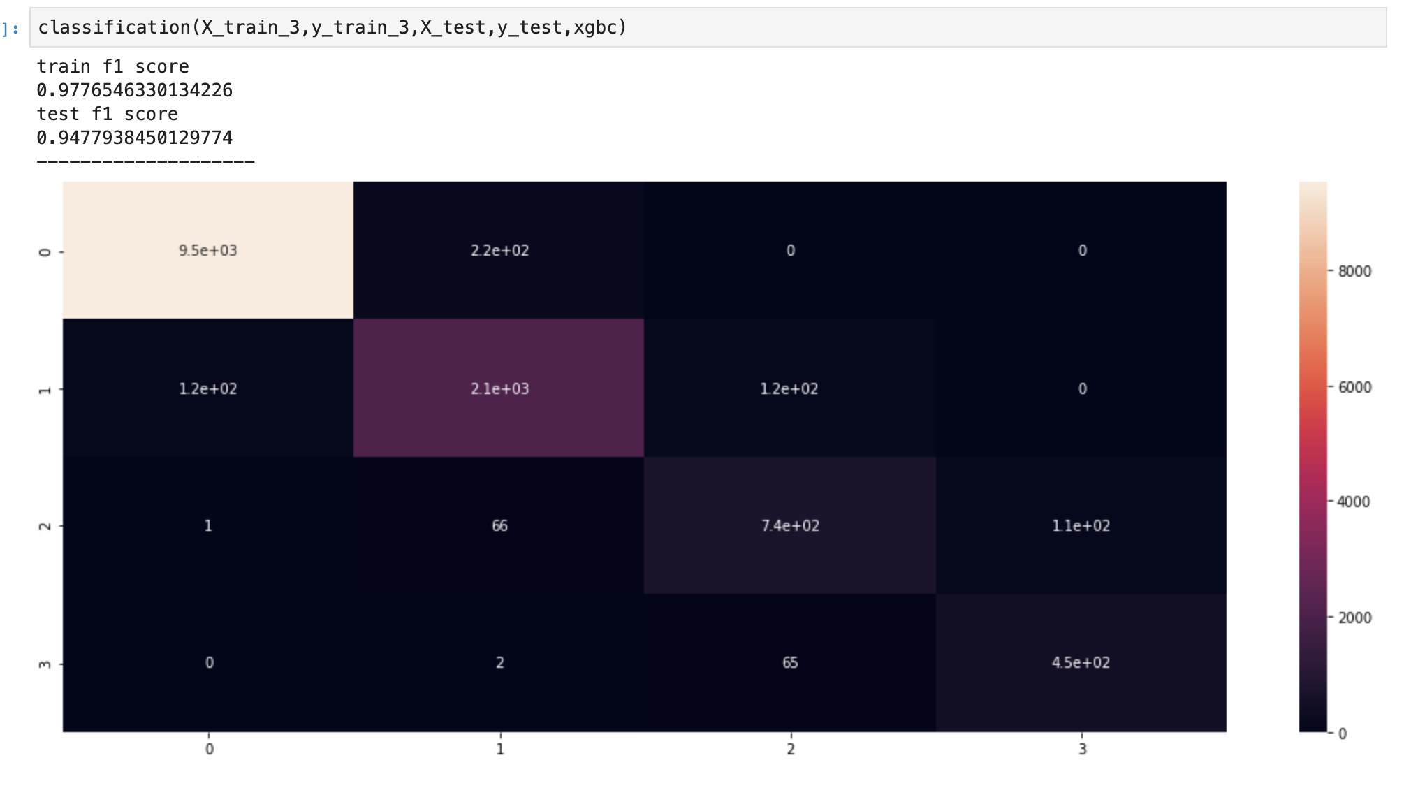
• It looks like we consistently improved our models as we progressed to more advanced methods of data balancing

Table of contents

---

8. What if we balance the test data also?

• I mainly ask this question as it will help reinforce what we saw above and instill confidence that our models are very strong
• Below, we start by balancing the test data

test = pd.concat([X_test,y_test],axis=1)

test_balanced = (upsample_classes(test,'price_bin'))

X_test_b = test_balanced.drop('price_bin',axis=1)
y_test_b = test_balanced.price_bin

• Below are the new outcomes following data balancing

Method 1

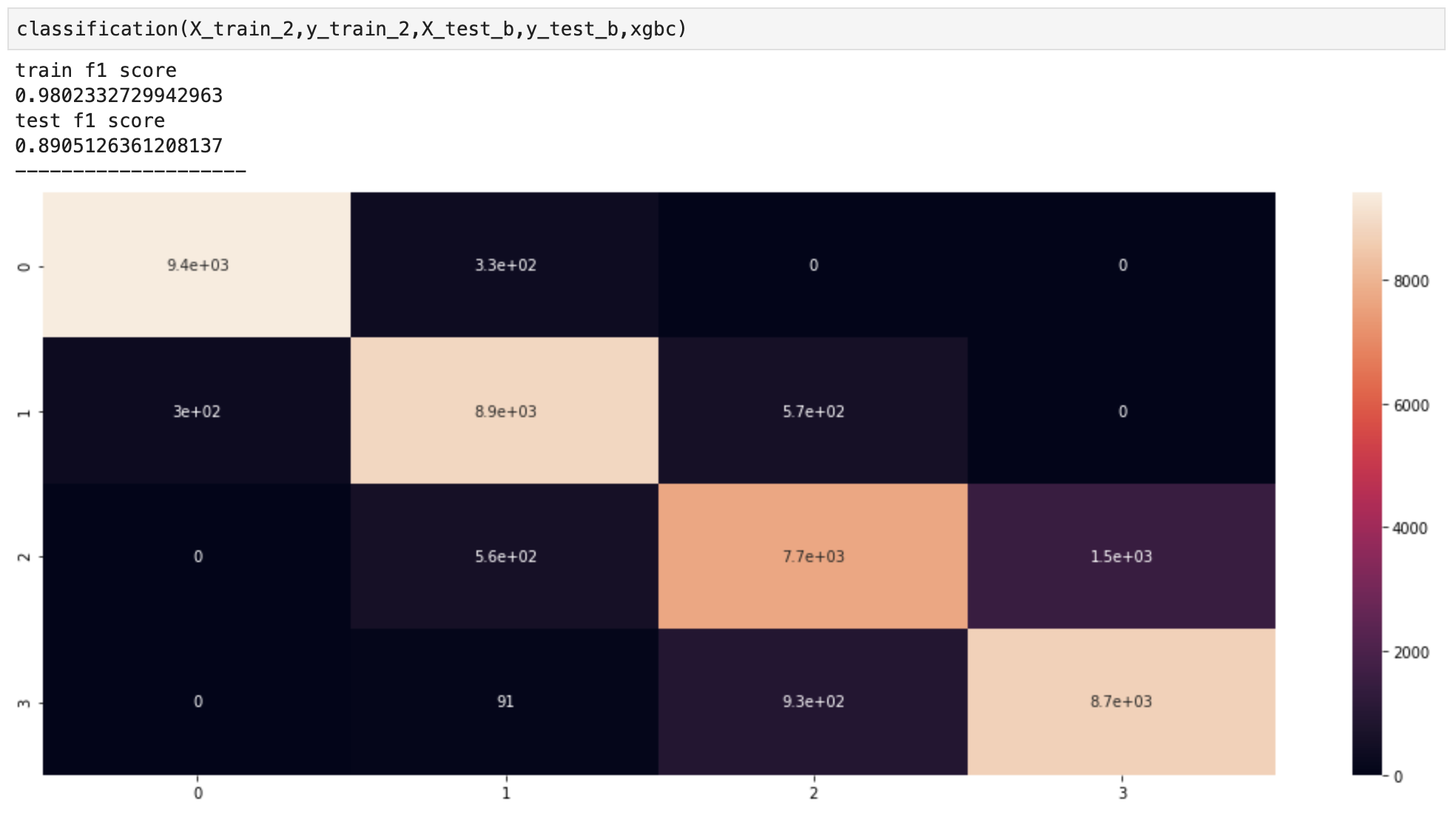
Method 2

Method 3

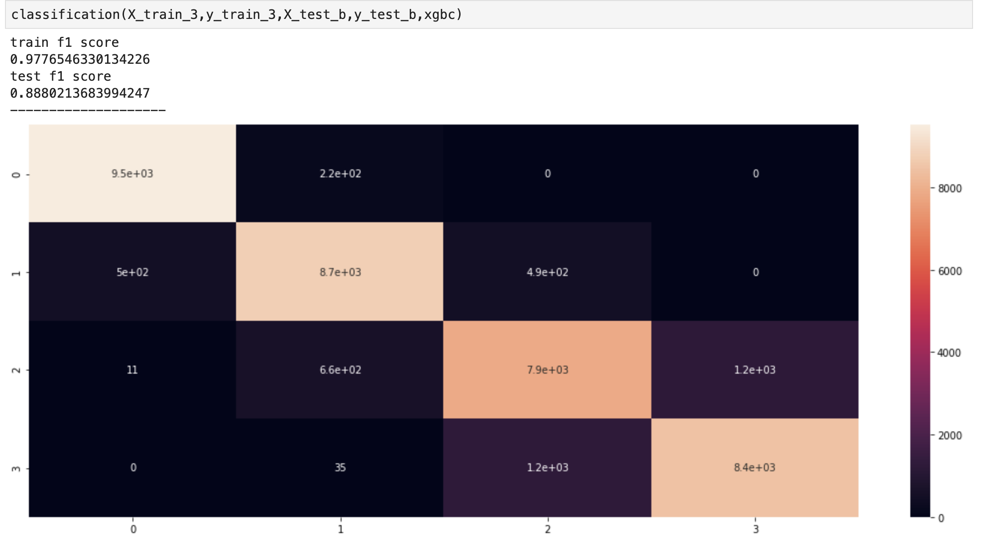
• Interestingly, method 2 slightly overtook SMOTE but SMOTE still managed to beat the most simple of the three options
• What we see here essentially confirms our observations above
• You may wonder what will happen as we introduce new data from each of the 4 diamond classes
• Above, we see what that would look like

Table of contents

---

9. Conclusion

Balancing data is often a key part of the Data Science process in classification algorithms. Conveniently, there are very simple, efficient, and effective ways to perform this crucial task. We saw the various types of ways and discussed the benefits and drawbacks of each style. We also explored the coding process we would use in python. I hope this post will help readers in their statistical inquiries to generate meaningful insights.

Table of contents

Thank you for taking time to read my post. I hope you learned something today.

10. Resources

Rane, C (2018). Diamonds In-Depth Analysis. Retrieved from https://www.kaggle.com/fuzzywizard/diamonds-in-depth-analysis

Testing Classification on Oversampled Imbalance Data.Retrieved from https://stats.stackexchange.com/questions/60180/testing-classification-on-oversampled-imbalance-data

Brwonlee, J (2020, January 17). SMOTE for Imbalanced Classification with Python. Retrieved from https://machinelearningmastery.com/smote-oversampling-for-imbalanced-classification/

Paul, S (2018, October 04). Diving Deep with Imbalanced Data. Retrieved from https://www.datacamp.com/community/tutorials/diving-deep-imbalanced-data

Murali, A (2018, May 31). Embed Code in Medium. Retrieved from: https://medium.com/@aryamurali/embed-code-in-medium-e95b839cfdda

Mahendru, K (2019, June 24). How to Deal with Imbalanced Data using SMOTE. Retrieved from https://medium.com/analytics-vidhya/balance-your-data-using-smote-98e4d79fcddb

Allien, M (2019, January 10). Creating Table of Contents for Medium Articles. Retrieved from https://medium.com/@AllienWorks/creating-table-of-contents-for-medium-articles-5f9087377b82#dc26

Doken, S (2017, November 06). SMOTE explained for noobs – Synthetic Minority Over-sampling Technique line by line. Retrieved from https://rikunert.com/SMOTE_explained

Lusa, L and Blagus, R (2013, March 22). Retrieved from: https://www.datacamp.com/community/tutorials/diving-deep-imbalanced-data

Table of contents