
Table of contents
- Why to use the Naive Bayes Classifier
- The data used
- How does Naive Bayes work for continuous features – GaussianNB
- How does Naive Bayes work for categorical features – CategoricalNB
- How does Naive Bayes work for binary features – BernoulliNB
- How does Naive Bayes work for multinomial features – MultinomialNB
- How does Naive Bayes work for multinomial features – ComplementNB
- Conclusion
- References
Why use the Naive Bayes Classifier
In a short answer, because Naive Bayes is simple, extremely fast, provides good results, is easy to implement in an IT production, is well suited when the training set does not fit in memory and is easy to explain in a regulatory industry. Naive Bayes is used for classification tasks (scoring, text & for imbalanced dataset) and it provides a good baseline for model comparison.
The algorithm is considered as simple (and as naive) because it is based on the assumption of the feature’s conditional independence which is rarely true in reality. For example, imagine you are trying to predict if a patient will do a cerebrovascular accident and you have these features: weight, levels of diabetes & cholesterol. We know that each one of these characteristics has an impact on the CVA and the more they increase, the more the CVA’s probability increases. However, Naive Bayes will consider these features as independent.
It is extremely fast due to the calculus to reach the decision’s probability for a class or another. We will see in detail in the "How…" parts but in simple words, it’s derived from the Bayes’ theorem in order to obtain a probability for each class. Then, the predicted class is the one having the highest probability (maximum a posteriori).
Despite its naive assumption it provides good results for classification because if we consider a loss function such as the zero-one loss, it does not penalize an inaccurate probability estimation as long as the maximum a posteriori‘s probability is assigned to the correct class. However, even if the label is well predicted, the probability itself does not have to be interpreted as a probability due to the never satisfied probability of independence. That is why it is really important to consider Naive Bayes as a classifier (binary or multiclass).
The calculus are simple to do (whatever the type of Naive Bayes you want to use) which make it easy to be implemented into a rules-based system decision engine. Therefore, it is an alternative to a logistic regression and a decision tree especially when dealing with multi-class target.
In some industries, it is not possible to use fancy & advanced Machine Learning algorithms due to regulatory constraints. Indeed, the calculus / results / the decision have to be explainable and this is what we will do in this article. Sklearn provides 5 types of Naive Bayes :
- GaussianNB
- CategoricalNB
- BernoulliNB
- MultinomialNB
- ComplementNB
We will go deeper on each of them to explain how each algorithm works and how the calculus are made step by step in order to find the exact same results as the sklearn’s output.
In case of large database that can’t be loaded in the memory, sklearn’s Naive Bayes functions have the _partialfit parameter. It can be very useful when we deal with textual data because we often face a sparse dataset who does not always fit in RAM.
To conclude, because Naive Bayes is widely studied since the 1960’s there are multiple adaptations in order to fit different kinds of data. Scikit-learn implemented it for continuous, multinomial, binomial and categorical types and we will see how to use them on a good way given the type of data we have.
The data used
For this article I will use a product sales related dataset where the objective is to classify "buy more than $X" vs "buy less than $X" given 3 features. I deliberately chose 3 features in order to explain easily how the Naive Bayes algorithms are working.
Originally these 3 features are continuous and I discretized them in order to use all the Naive Bayes’ algorithms in a right way.
The train dataset has 2.720 observations and the test set has 1.340 observations. Target = 1 (buy more than $X) for 50.3% of the train and 51% for the test so it is well balanced. Moreover, in the following examples, we will build the sklearn probabilities for these two observations named _two_obstest.

The original feature are X15, X16 and X18 but it is necessary to encode them in different ways given the chosen algorithm.
How does Naive Bayes work for continuous features – GaussianNB
In this part we will see step by step how the estimation of the a posteriori probability is made when we use the Gaussian Naive Bayes.
First of all, the Naive Bayes’ posterior probability calculus is defined as:

And because the evidence is a positive constant, it allows to normalize the results. In other words, it will not change any final decision and it allows to have the sum of the posterior probabilities equals to 1.
Let’s calculate the posterior probability for "buy more than $X" & "buy less than $X" for the observation 0 and 1 of the _two_obstest by using the variables X15, X16 and X18.
In our example the numerator has this form:

The estimation of the prior [e.g. P(buymore$X)] __ is very simple because it is the target rate:

Now the objective is to estimate the conditional probabilities [e.g. p(X15 | buy more than $X)] and we will use the equation of the Normal distribution:

So we need to compute for each class the mean and the variance (on Wikipedia the variance is estimated by the Bessel corrected variance. It tends to be equal to the variance when the number of observations increases because the variance is multiplied by n/(n-1) where n is the number of observations). NB: Sklearn implementation does not do this Bessel corrected variance.
Here is the estimation of the mean and the variance for each variable and for each class. Here, ddof (Delta Degree Of Freedom) = 0 because sklearn does not implement the Bessel corrected variance. If you want the same implementation as Wikipedia, you just have to replace ddof=0 by ddof=1.

We get the conditional probabilities by replacing these previous values into the Normal distribution of Figure7. For the observation 0 of _two_obstest (see the _two_obs_test[continuouslist].iloc[0,i] in the code where i is the position of the feature) the code of the conditional probabilities is:
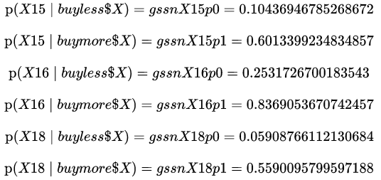
Now we have all the parameters to get the likelihood for the two classes + the evidence and we can calculate the a posteriori probabilities:
As a result the posterior probabilities for "buy more than $X" (gssnPbuymore in the above code) & "buy less than $X" (gssnPbuyless in the above code) for the observation 0 of _two_obstest are respectively 0.9945371191553004 and 0.005462880844699651. So, given that we take the argmax, 0.995 > 0.005 → gssnPbuymore > gssnPbuyless → we can consider the observation 0 as "buy more than $X" which is a good prediction as we see in Figure 4 !
If we do the same calculus for the values of the observation 1 (see Figure4) we will respectively obtain for "buy more than $X" (gssnPbuymore) & "buy less than $X" (gssnPbuyless) the values 0.008104869133118996 and 0.9918951308668811. So, given that we take the argmax, 0.008 < 0.992 → gssnPbuymore < gssnPbuyless → we can consider the observation 1 as "buy less than $X" which is as well a good prediction as we see in Figure4 !
Great, now let’s see how to get the exact same results with three lines of code with scikit-learn:
How does Naive Bayes work for categorical features – CategoricalNB
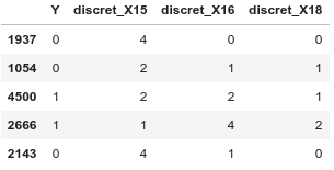
In this part we will see step by step how the estimation of the a posteriori probability is made when we use the Categorical Naive Bayes. In order to use the algorithm on a good way, you have to discretize your continuous features and several methods exists from the easiest to the most exotic one. Moreover, the categories has to be encoded by numbers from 0 to ni-1 where ni is the number of available categories for the feature i. After such transformation, the dataset looks like this:
The formula to estimate the conditional probabilities is:

Where Ntic is the number of times that a category t appears in the feature i into the class c. Nc is the size of sample for each class c. ni is the number of categories you have in the feature i. Then, alpha is a smoothing parameter (Laplace smoothing if 1 or Lidstone if ]0;1[ ). Alpha allows to have no issues in the calculus if you have a category with no observation in a class. Personally, I keep alpha=1 and tuning the parameter can bring a very marginal improvement.
Let’s calculate the a posteriori probability for "buy more than $X" & "buy less than $X" for the observation 0 and 1 of the _two_obstest by using the variables discret_X15, discret_X16 and discret_X18. The conditional probability of the observation 0 can be estimated with the following code:
Let me explain, we know on Figure3 that the value of the observation 0 for discret_X16 is 3. That is why I selected for the lines 5–6 the number of values equal to 3 for each class and +1 is for alpha. Then this numerator is divided by the number of observations in each class + (alpha {=1} multiplied by the number of categories in discret_X16 {=5}).
As a result, we have for each conditional probability:
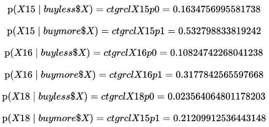
Now we have all the parameters to get the likelihood for the two classes + the evidence and we can calculate the posterior probabilities (NB: The priors are the same as Figure6.):
As a result the posterior probabilities for "buy more than $X" (ctgrclPbuymore) & "buy less than $X" (ctgrclPbuyless) for the observation 0 of _two_obstest are respectively 0.9886380451862543 and 0.01136195481374564. So, given that we take the argmax, 0.989 > 0.011 → ctgrclPbuymore > ctgrclPbuyless → we can consider the observation 0 as "buy more than $X" which is a good prediction as we see in Figure 4 !
If we do the same calculus for the values of the observation 1 (see Figure4) we will respectively obtain for "buy more than $X" (ctgrclPbuymore) & "buy less than $X" (ctgrclPbuyless) the values 0.020992001868815332 and 0.9790079981311848. So, given that we take the argmax, 0.021 < 0.979 → ctgrclPbuymore < ctgrclPbuyless → we can consider the observation 1 as "buy less than $X" which is as well a good prediction as we see in Figure4 !
Great, now let’s see how to get the exact same results with three line of code with scikit-learn:
How does Naive Bayes work for binary features – BernoulliNB
In this part we will see step by step how the estimation of the a posteriori probability is made when we use the Bernoulli Naive Bayes. To use the algorithm properly, you have to dummify the categorical features (with _pandas.get_dummies(dropfirst=False) for example). At the end, your database has to be composed by 0–1 only.
Keep in mind that if you don’t do the dummification or if you don’t transform your continuous features into a binary way, the algorithm implemented in sklearn will work from a calculating point of view but the results will be very bad. After such a transformation, the dataset looks like this:

The formula to estimate the conditional probabilities is:

If you want to go further, the calculus is well explained on the paper [1]
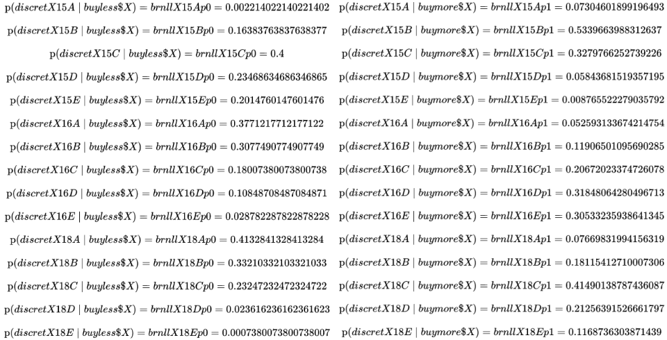
Let’s calculate the posterior probability for "buy more than $X" & "buy less than $X" for the observation 0 and 1 of the _two_obstest by using the variables discretX15…, discretX16… and discretX18… . The conditional probability of discret_X15_A can be estimated with the following code:
For the conditional probability knowing that Y=0 we have on the numerator the number of observations following the condition where discret_X15_A = 1 and Y = 0. Then we add the value 1 representing the Laplace smoothing. For the denominator, we count the number of the class’ observations which is the length of Y = 0 and we have +2 because we have two classes in the target. If it was a multinomial target having the values 0–1–2–3–4 then we would have +5.
As a result we have for each conditional probability:
Now we have all the parameters to get the likelihood for the two classes + the evidence and we can calculate the posterior probabilities (NB: The priors are the same as Figure6.):
We saw in Figure3. that the observation 0 has the value equals to 1 for _discret_X15B, _discret_X16D, _discret_X18D and the value equals to 0 for all the other _discret__ features. To compute the likelihood, we keep the conditional probability when the value equals to 1 and we multiply them by 1-conditionalProbability when the value equals to 0.
As a result the posterior probabilities for "buy more than $X" (brnllPbuymore) & "buy less than $X" (brnllPbuyless) for the observation 0 of _two_obstest are respectively 0.99586305749289 and 0.0041369425071100955. So, given that we take the argmax, 0.996 > 0.004 → brnllPbuymore > brnllPbuyless → we can consider the observation 0 as "buy more than $X" which is a good prediction as we see in Figure 4 !
If we do the same calculus for the values of the observation 1 (see Figure4) we will respectively obtain for "buy more than $X" (brnllPbuymore) & "buy less than $X" (brnllPbuyless) the values 0.0075457709306252525 and 0.9924542290693747. So, given that we take the argmax, 0.021 < 0.979 → brnllPbuymore < brnllPbuyless → we can consider the observation 1 as "buy less than $X" which is as well a good prediction as we see in Figure4 !
Great, now let’s see how to get the exact same results with three line of code with scikit-learn:
How does Naive Bayes work for multinomial features – MultinomialNB
In this part we will see step by step how the estimation of the a posteriori probabilities are made when we use the Multinomial Naive Bayes. To use the algorithm on a good way, we have to transform the database as we did for CategoricalNB or in any other numerical way (Spoiler alert: it is perfectly adapted for counting features). The estimation of the conditional probabilities are obtained with this formula:
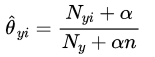
Nyi represents the sum of the values for the class y and the feature i + the Laplace parameter. For the denominator, Ny represents the overall sum of all the values in the database for the class y + alpha to be multiplied by n which represents the number of features used (without the target).
We clearly see something strange if we want to apply this formula to our discretized database like the one used for categoricalNB. The strange thing comes from the Nyi & Ni because they are the sum of the values and not the length. Which means that the way we give a value to the category (like 0–1–2-… or 1–3–5-…) will have an impact on both the sums in the numerator and denominator which will impact the overall calculus and make it suboptimal. As a result, the Multinomial Naive Bayes is widely used for text classification where we have counting data like Bag of Words or TFIDF. In our case and with our kind of data, it would be smarter to one hot encode our discretized data and then to apply the Multinomial Naive Bayes. Spoiler alert: as we will see just afterwards, doing a Multinomial Naive Bayes on one hot encoded data provides the exact same results than the Categorical Naive Bayes.
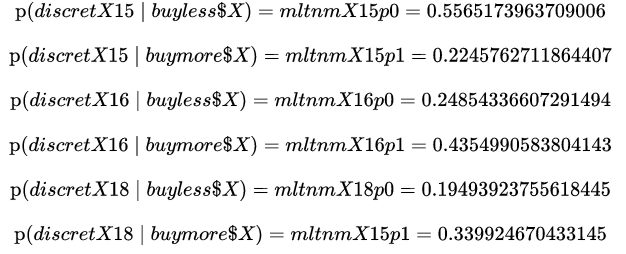
Now, let’s show how the Multinomial Naive Bayes a posteriori‘s probabilities are obtained. In order to avoid to much code & Latex I will provide the results of the calculus for the discretized data and not the one hot encoded as it should be. The two Priors remain the same as before, we get the conditional probabilities:
The first line aims to get the conditional probability of discret_X15 for the class 0. The merge and the sum allow to obtain the sum of all values of discret_X15 that are in the class 0 and +1 is the alpha. For the denominator, the merge followed by a sum of a sum allows to get the sum of all of the elements in the database for the class 0; +3 (in reality +3*alpha) represents the 3 features that we use (discret_X15, discret_X16 & discret_X18). The results of each conditional probabilities are:
We now have all the parameters to get the likelihood for the two classes + the evidence and we can calculate the posterior probabilities (NB: The priors are the same as Figure6.):
We saw in Figure3. that the observation 0 has the value 1 for _discretX15, the value 3 for _discretX16 and the value 3 for _discretX18. Indeed that is why we have the likelihood equals to the conditional probability of discret_X15 to the first multiplied by the conditional probability of discret_X16 cubed multiplied by the conditional probability of discret_X18 cubed.
As a result the posterior probability for "buy more than $X" (mltnmPbuymore) & "buy less than $X" (mltnmPbuyless) for the observation 0 of _two_obstest are respectively 0.9208203346956907 and 0.0791796653043093. Therefore, given that we take the argmax, 0.921 > 0.079 → mltnmPbuymore > mltnmPbuyless → we can consider the observation 0 as "buy more than $X" which is a good prediction as we see in Figure 4 !
If we do the same calculus for the values of the observation 1 (see Figure4) we will respectively obtain for "buy more than $X" (mltnmPbuymore) & "buy less than $X" (mltnmPbuyless) the values 0.14128331134420608 and 0.8587166886557939. So, given that we take the argmax, 0.141 < 0.859 → mltnmPbuymore < mltnmPbuyless → we can consider the observation 1 as "buy less than $X" which is as well a good prediction as we see in Figure4 !
Great, now let’s see how to get the exact same results with three line of code with scikit-learn:
However, as I said earlier in this chapter, it is not relevant to use the discretized features for Multinomial Naive Bayes if it is not counting data. That is why it is better to use one hot encoded data like this:
And this provides exactly the same results as the Categorical Naive Bayes both for binary & multiclass classification.
How does Naive Bayes work for multinomial features – ComplementNB
Complement Naive Bayes [2] is the last algorithm implemented in scikit-learn. It is very similar to Multinomial Naive Bayes due to the parameters but seems to be more powerful in the case of an imbalanced dataset. Like Multinomial Naive Bayes, Complement Naive Bayes is well suited for text classification where we have counting data, TFIDF, … Like in the previous part, we will see step by step how the estimation of the a posteriori probabilities are made when we use the Complement Naive Bayes. To use the algorithm on a good way, you have to transform your database as you did for MultinomialNB. The estimation of the conditional probabilities is obtained with the following calculus:
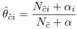
Where Nc̃i represents the sum of the values for the other classes c in the feature i + the Laplace parameter. For the denominator, Nc̃ represents the overall sum of all the values in the database for the other classes c + alpha which represents the number of features used (without the target). To illustrate what "other classes" mean, imagine (in a binary classification) that you want the conditional probability of a feature knowing the class 0 so you will do the sum of the values when the target=1. As a result, the conditional probabilities are the "opposite" of the Multinomial Naive Bayes ones in the case of a binary classification. In the paper, the authors advocate to normalize the conditional probabilities because the independence assumption would affect the final results especially in text classification. Sklearn implements the normalization has a True/False parameter.
The code shows that the calculus is "the same" as the Multinomial Naive Bayes one and this time I multiplied the conditional probabilities by -np.log in order to provide another way to get the final a posteriori probabilities:
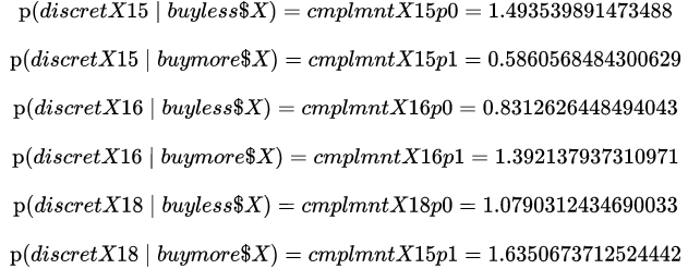
NB: If you put the normalizing parameter as True in sklearn (norm=True), the value of the conditional probabilities will be :
Once we have our conditional probabilities, I integrate them in a matrix (2D array):
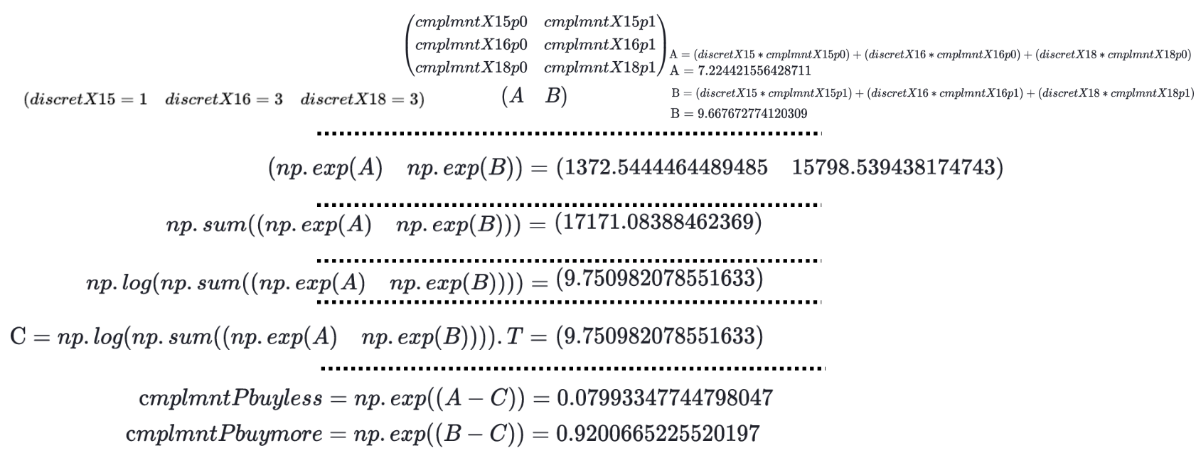
As a result, the posterior probabilities for "buy more than $X" (cmplmntPbuymore) & "buy less than $X" (cmplmntPbuyless) for the observation 0 of _two_obstest are respectively 0.9200665225520197 and 0.07993347744798047. Therefore, given that we take the argmax, 0.920 > 0.080 → cmplmntPbuymore > cmplmntPbuyless → we can consider the observation 0 as "buy more than $X" which is a good prediction as we see in Figure 4 !
If we do the same calculus for the values of the observation 1 (see Figure4) we will respectively obtain for "buy more than $X" (cmplmntPbuymore) & "buy less than $X" (cmplmntPbuyless) the values 0.14003899976530304 and 0.8599610002346968. So, given that we take the argmax, 0.140 < 0.960 → cmplmntPbuymore < cmplmntPbuyless → we can consider the observation 1 as "buy less than $X" which is as well a good prediction as we see in Figure4 !
Great, now let’s see how to get the exact same results with three line of code with scikit-learn:
However, as we see before, it is not relevant to use the discretized features for Complement Naive Bayes if it is not counting data. That is why it is better to use one hot encoded data like this:
And this provides exactly the same results has the one of Categorical Naive Bayes & Multinomial Naive Bayes due to the binary target.
Conclusion
We saw why the Naive Bayes algorithms can be used in a regulated industry where the calculus leading to a decision has to be explainable. More widely, they provide a good classification baseline for both numerical & textual data types and they are easy to implement with or without Python.
We saw how to use properly each algorithm given the data types we have and how they work step by step + how to use them within sklearn.
References
[1]: Andrew McCallum , Kamal Nigam(1998). A comparison of event models for Naive Bayes text classification.
[2]:Rennie, J. D., Shih, L., Teevan, J., & Karger, D. R. (2003). Tackling the poor assumptions of naive bayes text classifiers. In ICML (Vol. 3, pp. 616–623).


