Getting Started
Null values will always be the ire of the data scientist and managing them correctly can be the difference between an application that breaks and an application that soars.
This is particularly important with GIS images, or any rasterized data. We cannot ignore nulls or fill them with zeros (removing is not an option!) because it would produce unsightly holes in the resulting image (see example below).

We must apply a technique called spatial filtering to fill nulls with information that reflects the context or surroundings in which we find them.
In order for the "AFTER" image (above) to appear consistent or smooth, we know that a null pixel from the top of the "BEFORE" image should be filled with a very different value than a null found in the bottom of the image. **** So, how can we calculate these new values appropriately and systematically using Python?
Check out the full code for this project on my Github page (link).
A data engineering task
My colleague Daniel Bonhaure and I built a pretty standard GIS analytics web application that allows users to upload vector datasets (i.e. shapefiles), visualize them and perform analysis on the stored data. However, before storing the data in the database our data engineering pipeline must properly deal with the nulls.
If I were writing this about the R programming language, this would be a much shorter article because R provides one simple function, focal(), that does it all. However, with Python, it’s a harder nut to crack. We will need to summon the powers of NumPy, SciPy and Matplotlib.
It’s convoluted… in a good way
Spatial filtering or focal analysis is a technique of map algebra where we use the values of neighboring pixels to alter the values of a target pixel, in our case a null value. If you have ever used an image filter to beef up your Instagram photo, this is that exact same technique.

She has many names – window, kernel, filter footprint, map – but essentially it’s a two-dimensional array (most commonly either 3 x 3 or 5 x 5) that travels pixel-by-pixel across the image, where each pixel in the dataset has a turn in the center, i.e. the fifth or position x[4] in our 3 x 3 array. This process is called convolution.
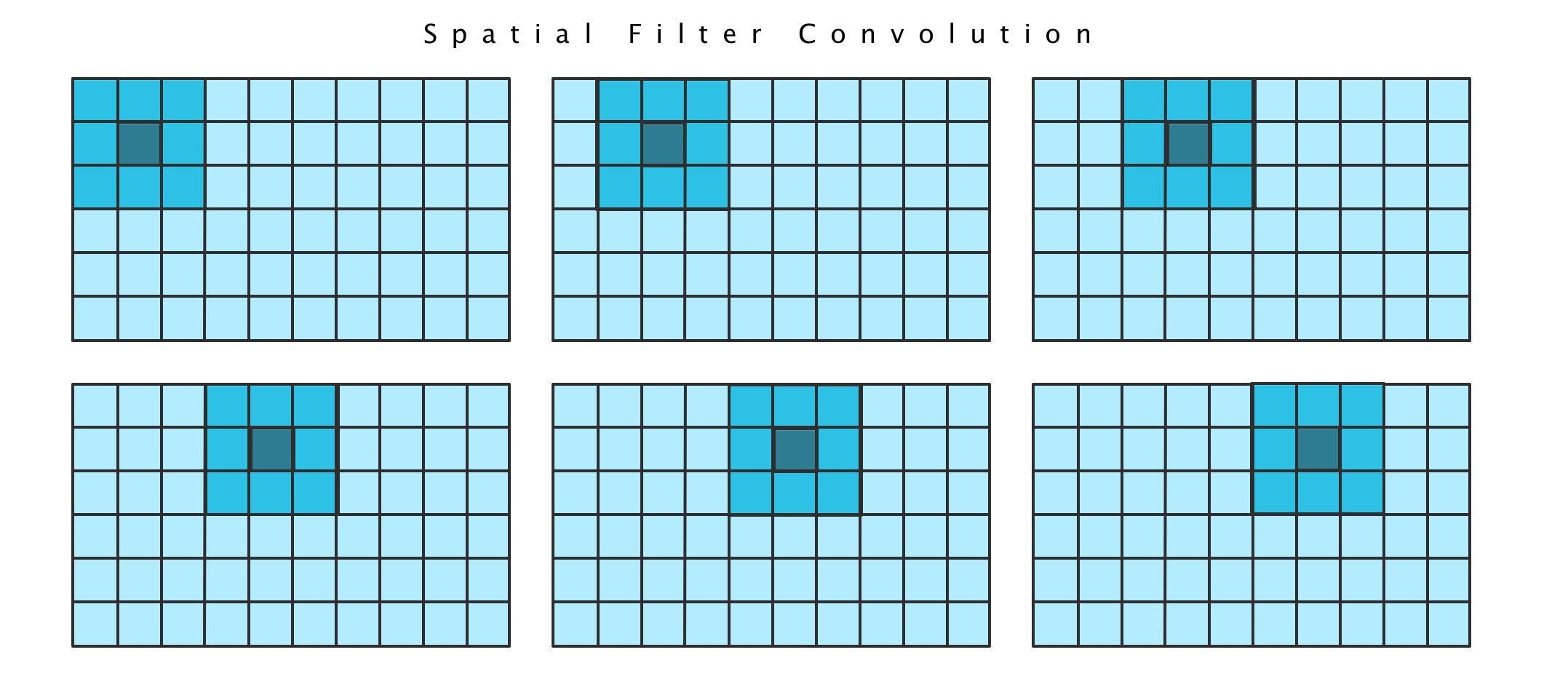
The filter that we used in our function only fires when a null value is found in the target position i.e. x[4]. When found, it fills that value with the mean of the surrounding pixels.
The SciPy multi-dimentional Image Processing submodule offers several options for convolution and filtering; we used generic_filter() in our system (see below).
Edge cases
If you check out the notebook you will see that our filter window works great, but we have skipped over a very important detail: the edge. That is, what do we do when the target value of our filter window is on the border of our raster matrix?
This is handled by the mode parameter in the SciPy generic_filter() function, which offers five options:

- constant – extends the values of the window by filling it with whatever we pass into the cval parameter; in our case cval=np.NaN.
- reflect – repeats values near the outside edge but in opposite order (with a 3 x 3 window this would include just the pixels at the edge of the raster; a 5 x 5 would include two additional reflected values).
- nearest – takes the values closest to the edge only (with a 3 x 3 window this is equivalent to reflect).
- mirror – extends the values of the window beyond the raster edge in a reflective pattern of the inner matrix but skipping the edge values (in a 3 x 3 matrix this means the added row or column is not the edge but the second from the edge).
- wrap – extends the values of the window by taking the values from the opposite side of the matrix (like in Super Mario when you jump out one side of the screen and appear on the other)
Advanced filter algorithms
Now that we have successfully smoothed our nulls using spatial filtering, why not take this a step further. Using the same pipeline, we can apply any spatial algorithm we want by adding it to our generic_filter() function.
In this example, because we are using a digital elevation model or DEM, it might be logical to calculate the slope at each point in the plot. We can do this using the neighborhood algorithm (below).

The dataset we are looking at is farmland (pretty flat) so the slope graph is not terribly exciting, …but you get the idea.
Conclusion
The solution presented here for cleaning raster data – spatial filtering – is particular to the science of image processing and requires specialized knowledge of map algebra and convolution.
Although spatial filtering is a somewhat involved method for smoothing nulls, we can repurpose this same technique to apply more sophisticated scientific calculations on our data, such as calculating the slope of a digital elevation model at each point.
🔥🔥🔥🔥
Further reading:
- Chris Garrard, Geoprocessing with Python (2016)
- The Neighborhood Algorithm, Penn State University


