How to vectorize pairwise (dis)similarity metrics

Hands-on Tutorials

You can vectorize a whole class of pairwise (dis)similarity metrics with the same pattern in NumPy, PyTorch and TensorFlow. This is important when a step inside your Data Science or machine learning algorithm requires you to compute these pairwise metrics because you probably don’t want to waste compute time with expensive nested for loops.

This pattern works any time you can break the pairwise calculation up into two distinct steps: expand and reduce. And it works equally well for similarity metrics like intersection over union between two boxes and dissimilarity metrics like Euclidean distance. This post explains the pattern and makes it concrete with two real-world examples.

For brevity, I sometimes refer to "similarity" as a shorthand for both similarity and dissimilarity. I also sometimes use "point" to mean any item we might use in pairwise comparisons. For example, in computer vision, a box encoded as (x1, y1, x2, y2) can be treated as a point in 4-dimensional space.

Why do we calculate pairwise similarity functions?

There are several data science and Machine Learning algorithms that require pairwise similarity metrics as one of their steps. Indeed, scikit-learn has an entire module dedicated to this type of operation.

Here are a few examples where you might want to compute pairwise metrics:

• Comparing points to centroids. In both clustering and classification, it can be useful to compare individual points to the class means for a set of points. These class mean values are called centroids and they are themselves points, which means the comparison is a pairwise operation.
• Creating cost matrices for bipartite assignment. In tracking-by-detection, you typically want to assign new detections to existing objects by similarity. The Hungarian algorithm can create these assignments by minimizing total cost while requiring that one object gets assigned to one detection (at most) and vice versa. The input to that algorithm is a cost matrix where each element is the dissimilarity between an object and a new detection. Examples of dissimilarity could be Euclidean distance or the inverse of Intersection over Union.
• Creating kernels for Gaussian process (GP) regression. The uncertainty in a Gaussian process is defined by a function that parameterizes the covariance between arbitrary pairs of points. Doing inference with a GP requires you to compute a matrix of pairwise covariance for your dataset. The most common covariance function is the squared exponential.

Why is pairwise similarity a bottleneck?

By "pairwise", we mean that we have to compute similarity for each pair of points. That means the computation will be O(M*N) where M is the size of the first set of points and N is the size of the second set of points. The naive way to solve this is with a nested for-loop. Don’t do this! Nested for loops are notoriously slow in Python.

The beauty of Numpy (and its cousins PyTorch and TensorFlow) is that you can use vectorization to send for loops to optimized, low-level implementations. Writing fast, scientific Python code is largely about understanding the APIs of these packages.

So how does it work?

Typically, if you want to vectorize a pairwise similarity metric between a set of M D-dimensional points with shape (M, D) and a set of N D-dimensional points with shape (N, D), you need to perform two steps:

1. Expand. Use an element-wise operation between two D-dimensional points with broadcasting to produce an expanded array with shape (M, N, D).
2. Reduce. Use an aggregate operation to reduce the last dimension, creating a matrix with shape (M, N).

It’s pretty simple. There are just a couple things to be aware of:

• When you compute pairwise similarity between a matrix of points and itself, M will be the same as N.
• Sometimes you will want to apply additional element-wise calculations for your similarity metric as well. This can be done anytime without messing up the result.

Let’s look at a few examples where we compute pairwise similarity between sets of points and themselves to make the process more concrete.

Pairwise Manhattan distance

We’ll start with pairwise Manhattan distance, or L1 norm because it’s easy. Then we’ll look at a more interesting similarity function.

The Manhattan distance between two points is the sum of the absolute value of the differences. Say we have two 4-dimensional NumPy vectors, x and x_prime. Computing the Manhattan distance between them is easy:

import numpy as np

x = np.array([1, 2, 3, 4])
x_prime = np.array([2, 3, 4, 5])

np.abs(x - x_prime).sum()

# Expected result
# 4

Now, we’ll extend Manhattan distance to a pairwise comparison. Let X be the four corners of a unit square:

X = np.array([
    [0, 0],
    [0, 1],
    [1, 1],
    [1, 0]
])

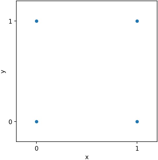
The Manhattan distance between any pair of these points will be 0 (if they’re the same), 1 (if they share a side) or 2 (if they don’t share a side). A pairwise dissimilarity matrix comparing the set of points with itself will have shape (4, 4). Every point gets a row and every point gets a column. The order of the rows and columns will be the same, which means we should get 0s along the diagonal since the Manhattan distance between a point and itself is 0.

Let’s compute pairwise Manhattan distance between each of these points and themselves the naive way, with a nested for-loop:

manhattan = np.empty((4, 4))

for i, x in enumerate(X):
    for j, x_prime in enumerate(X):
        manhattan[i, j] = np.abs(x - x_prime).sum()

manhattan

# Expected result
# array([[0., 1., 2., 1.],
#        [1., 0., 1., 2.],
#        [2., 1., 0., 1.],
#        [1., 2., 1., 0.]])

Every element manhattan[i, j] is now the Manhattan distance between point X[i] and X[j]. Easy enough.

Now, let’s vectorize it. The first thing we need is an expand operation that can be broadcast over pairs of points to create a (4, 4, 2) array. Subtraction works with broadcasting so this is where we should start.

To expand correctly, we need to insert dimensions so that the operands have shape (4, 1, 2) and (1, 4, 2) respectively. This works because NumPy broadcasting steps backwards through the dimensions and expands axes when necessary. This will result in a distance array that is (4, 4, 2):

deltas = X[:, None, :] - X[None, :, :]
deltas.shape

# Expected result
# (4, 4, 2)

Now we’ve created a 4×4 set of 2-dimensional points called deltas. The way this result works is that deltas[i, j, k] is the result of X[i, k] - X[j, k]. It would be equivalent to assigning deltas[i, j, :] = x - x_prime in the nested for loop above.

At this point, we’re free to apply the element-wise absolute value operation since it doesn’t change the shape:

abs_deltas = np.abs(deltas)
abs_deltas.min()

# Expected result
# 0

We still need to perform the reduce step to create (4, 4) L1 distance matrix. We can do this by summing over the last axis:

manhattan_distances = abs_deltas.sum(axis=-1)
manhattan_distances

# Expected result
# array([[0, 1, 2, 1],
#        [1, 0, 1, 2],
#        [2, 1, 0, 1],
#        [1, 2, 1, 0]])

Voila! Vectorized pairwise Manhattan distance.

By the way, when NumPy operations accept an axis argument, it typically means you have the option to reduce one or more dimensions. So, to go from a (4, 4, 2) array of deltas to a (4, 4) matrix with distances, we sum over the last axis by passing axis=-1 to the sum() method. The -1 is shorthand for "the last axis".

Let’s simplify the above snippets to a one-liner that generates pairwise Manhattan distances between all pairs of points on the unit square:

np.abs(X[:, None, :] - X[None, :, :]).sum(axis=-1)

# Expected result
# array([[0, 1, 2, 1],
#        [1, 0, 1, 2],
#        [2, 1, 0, 1],
#        [1, 2, 1, 0]])

Pairwise Intersection over Union

Now that you’ve seen how to vectorize pairwise similarity metrics, let’s look at a more interesting example. Intersection over Union (IoU) is a measure of the degree to which two boxes overlap. Assume you have two boxes, each parameterized by its top left corner (x1, y1) and bottom right corner (x2, y2). IoU is the area of the intersection between the two boxes divided by the area of the union between the two boxes.

Let’s use boxes generated from the popular YoloV3 model. We’ll use relative coordinates so the maximum possible value for any of the coordinates is 1.0 and the minimum is 0.0:

bicycle = np.array([0.129, 0.215, 0.767, 0.778])
truck = np.array([0.62 , 0.141, 0.891, 0.292])
dog = np.array([0.174, 0.372, 0.408, 0.941])

The area of a box (x1, y1, x2, y2) is (x2 - x1) * (y2 - y1). So if you have two boxes a and b, you can compute IoU by creating an intersection box (when it exists) and then calculating the area of the intersection, and the area of each of the individual boxes. Once you have that, IoU is intersection / (a_area + b_area - intersection). The result will be 0 if the boxes don’t overlap (because the intersection box doesn’t exist) and 1 when the boxes have perfect overlap.

Here’s the code to calculate IoU for the bicycle-dog pair and the dog-truck pair:

def iou(a, b):
    """
    Intersection over Union for two boxes a, b
    parameterized as x1, y1, x2, y2.
    """
    # Define the inner box
    x1 = max(a[0], b[0])
    y1 = max(a[1], b[1])
    x2 = min(a[2], b[2])
    y2 = min(a[3], b[3])
    # Area of a, b separately
    a_area = (a[2] - a[0]) * (a[3] - a[1])
    b_area = (b[2] - b[0]) * (b[3] - b[1])
    total_area = a_area + b_area
    # Area of inner box
    intersection = max(0, x2 - x1) * max(y2 - y1, 0)
    # Area of union
    union = total_area - intersection
    return intersection / union

iou(bicycle, dog), iou(dog, truck)

# Expected result
# (0.2391024221313951, 0.0)

In order to vectorize IoU, we need to vectorize the intersection and total area separately. Then we can calculate IoU as an element-wise operation between the two mat

First, stack the three boxes to create a (3, 4) matrix:

X = np.stack([
    dog,
    bicycle,
    truck
])
X.shape

# Expected result
# (3, 4)

The np.stack() operation puts multiple NumPy arrays together by adding a new dimension. By default, it adds a dimension at the beginning.

Next, compute the coordinates of the intersection boxes for all pairs of boxes:

x1 = np.maximum(X[:, None, 0], X[None, :, 0])
y1 = np.maximum(X[:, None, 1], X[None, :, 1])
x2 = np.minimum(X[:, None, 2], X[None, :, 2])
y2 = np.minimum(X[:, None, 3], X[None, :, 3])

inner_box = np.stack([x1, y1, x2, y2], -1)
inner_box.shape

# Expected result
# (3, 3, 4)

This is the expand step for intersection. We can’t do it in a single step because the inner box is the maximum between corresponding coordinates and the minimum between others. But we stack the result to make it clear that this step indeed expands the result to a (3, 3, 4) array. Each element inner_box[i, j, k] is the kth coordinate of the intersection between box i and box j.

Now, calculate the area of the inner box:

intersection = (
    np.maximum(inner_box[..., 2] - inner_box[..., 0], 0) *
    np.maximum(inner_box[..., 3] - inner_box[..., 1], 0)
)
intersection.shape

# Expected result
# (3, 3)

The area operation reduces the last dimension. We’re doing that reduction manually by selecting indices, but we are still reducing that dimension, just like we did with sum(axis=-1) above.

We need to do another pairwise operation to get total area between pairs of boxes, but this one is a little different. For total area, the "points" are no longer boxes, they are areas. That is, instead of doing a pairwise calculation between two (3, 4) sets of boxes, we will do a pairwise operation between two sets of areas. Although we’re stretching the term "point", the pattern is the same as the previous examples.

First, we compute the area of each individual box to create our area vectors, then we compute total area with an expand step:

a_area = (X[:, 2] - X[:, 0]) * (X[:, 3] - X[:, 1])
b_area = (X[:, 2] - X[:, 0]) * (X[:, 3] - X[:, 1])

total_area = a_area[:, None] + b_area[None, :]
total_area.shape

# Expected result
# (3, 3)

Think of total_area as having shape (3, 3, 1) where each element total_area[i, j, 0] contains the sum of the areas between a pair of boxes. NumPy squeezes the last dimension automatically, so the actual result is (3, 3) and we don’t need to explicitly perform the reduce step.

The rest of the IoU calculation is element-wise between the intersection and total_area matrices. This is analogous to the single box case above:

union = total_area - intersection
intersection / union

# Expected result
# array([[1.        , 0.23910242, 0.        ],
#        [0.23910242, 1.        , 0.02911295],
#        [0.        , 0.02911295, 1.        ]])

Notice, the diagonal elements are all 1 (perfect IoU) and the non-overlapping elements are all 0.

Conclusion

That’s it! In this post, we talked about what pairwise similarity is and some use cases where it’s important. We also talked about why it can be such a bottleneck for your machine learning algorithms. Then, we saw a general approach to vectorizing these pairwise similarity computations: 1) expand and 2) reduce. If you can break the pairwise calculation up into these two steps then you can vectorize it. And you’re free to add any additional element-wise operations you might need. All the examples in this post used NumPy, but don’t forget that you can use this trick in PyTorch and TensorFlow as well.

Happy programming!